Tag: RKNN-Toolkit2

  • Anima RKNN Inference Optimization: Reducing Generation Time by 41% with Spectrum

    Anima RKNN Inference Optimization: Reducing Generation Time by 41% with Spectrum

    Affiliate Disclosure: This post contains AliExpress affiliate links. If you make a purchase through these links, the author may receive a commission.

    1. Reducing Image Generation Time

    When running large-scale Diffusion Transformers (DiT) on-device in a single-board computer (SBC) environment, memory constraints and computation time are the primary bottlenecks. Using a Radxa ROCK 5C 8GB board purchased directly from the official Radxa AliExpress store, we conducted Anima DiT inference optimization experiments based on the 2026-8 environment.

    Denoising a 512×512 image for 20 steps took 2,408.54 seconds. Including the time required to reconstruct the image with the VAE, generating a single image exceeded 30 minutes. A method was needed to reduce the computational workload while preserving the visual quality of the output.

    We applied Spectrum to the FP16 RKNN configuration executed in Part 1. While retaining the Euler scheduler, we replaced model computations on selected steps with predictions based on prior results, and compared the speed and image quality.

    2. Hardware and Model Configuration Used for Comparison

    The experimental hardware is the Radxa ROCK 5C single-board computer, equipped with a Rockchip RK3588S2 SoC and 8GB of system memory.

    The RKNN runtime target is rk3588. The test device is the ROCK 5C 8GB, which must be distinguished from the ROCK 5C Lite listed on the same product page.

    We used 84 FP16 RKNN models, partitioning Anima’s 28 DiT blocks into self-attention, cross-attention, and FFN subgraphs. The underlying conversion structure is identical to the setup described in Part 1.

    The NPU processes primary matrix and attention operations. The CPU handles AdaLN, FP32 residual accumulation, the Euler scheduler, text encoding, and VAE decoding. This division of roles was maintained even after adding Spectrum.

    3. What Computations Does Spectrum Skip?

    Spectrum is not a sampler that replaces Euler. It is a caching technique that predicts the denoised state of the current step from prior computational results to reduce model recalculations. We ported the Spectrum implementation from stable-diffusion.cpp to NumPy and integrated it into the Euler loop.

    The core principle of Spectrum leverages the property that latent variable trajectories do not change abruptly between steps during diffusion, forecasting an estimate of the denoised state \(x_0\) from a prior history buffer.

    At each step, the pipeline selects between direct computation and prediction. Both paths feed their results into the same Euler scheduler.

    • On directly computed steps, conditional and unconditional outputs are combined via CFG, and the denoised state is calculated as x₀ = xₜ − σ × prediction and stored in the history buffer.
    • On prediction steps, the current x₀ is estimated from prior history, skipping NPU model computation entirely.
    • The estimated x₀ is converted back into a flow prediction via prediction = (xₜ − x₀) / σ. Both paths update the next state using the same Euler integrator.

    Thanks to this architecture, the scheduler itself retains the FlowMatch Euler formulation while substantially reducing the number of tensor operations dispatched to the NPU.

    4. 20 Steps: 11 Computations, 9 Predictions

    Across a 20-step run, the steps computed directly and those replaced with predictions are broken down as follows:

    • Actual model computation steps (11 steps): Step 1, 2, 3, 4, 6, 8, 11, 14, 18, 19, 20
    • State prediction skipped steps (9 steps): Step 5, 7, 9, 10, 12, 13, 15, 16, 17

    The first 4 steps were all directly computed to accumulate the history required for forecasting. In the intermediate phase, 9 steps were replaced with predictions, and the final 18~20 step was directly computed again.
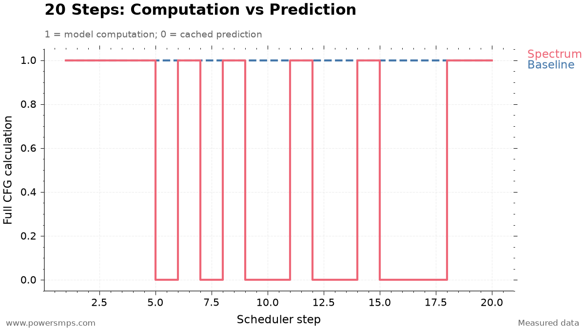
    20-Step Sampling Policy: Baseline vs Spectrum Forecasting
    20-Step Sampling Policy: Baseline vs Spectrum Forecasting

    Here, 11 computation steps do not translate to just 11 NPU executions. Each CFG step requires separate DiT evaluations for conditional and unconditional inputs.

    Because each transformer evaluation traverses 84 RKNN subgraphs across 28 blocks, 1 CFG evaluation requires 168 subgraph NPU executions (84 × 2). Therefore, the 11 model computations in the Spectrum pipeline represent the following actual hardware traversal volume:

    • Full model passes (Transformer Passes): 11 passes × 2 = 22 passes
    • Subgraph NPU execution count: 11 passes × 2 × 84 subgraphs = 1,848 executions

    By contrast, the baseline pipeline executes 40 transformer passes and 3,360 subgraph NPU executions across 20 steps. In other words, Spectrum eliminated exactly 18 model passes and 1,512 subgraph executions, significantly cutting hardware load.

    5. Benchmark Results: Total Generation Time Reduced by 41.02%

    The baseline and Spectrum were evaluated on the same ROCK 5C 8GB. The resolution (512×512), 20 steps, CFG scale of 4.0, and seed 20260812 were kept strictly identical.

    Metric Baseline Non-cached FP16 RKNN + sd-cpp VAE Spectrum Accelerated Pipeline Difference & Speedup
    20-Step Denoise Latency 2,408.54 seconds 1,356.58 seconds 1,051.96 seconds saved (43.68% reduction, 1.775× speedup)
    sd-cpp Tiled CPU VAE Decoding 155.04 seconds 155.46 seconds +0.42 seconds (comparable run-to-run variance)
    Total Elapsed Time (Excluding Prompt Encoding) 2,563.58 seconds 1,512.04 seconds 1,051.54 seconds saved (41.02% reduction, 1.695× speedup)

    The measured figures highlight the following bottleneck and optimization characteristics:

    1. Concentration of Denoising Acceleration: Net 20-step denoise latency decreased from the baseline of 2,408.54 seconds to 1,356.58 seconds with Spectrum, saving 1,051.96 seconds. This represents a 43.68% time reduction and a 1.775× speedup. This achieves near-linear acceleration efficiency, closely matching the proportion of skipped operations (45%, or 9 out of 20 steps).
    2. Independence of VAE Decoding: The lightweight tiled CPU VAE decoder from sd-cpp, powered by ARM NEON/OpenMP via the ggml backend, took 155.04 seconds for the baseline and 155.46 seconds for the Spectrum pipeline—a difference of just 0.42 seconds. In this benchmark, VAE decoding time remained essentially identical, confirming that the performance gains were concentrated almost exclusively in the denoising stage.
    3. Full-Pipeline Speedup: Excluding prompt encoding, total end-to-end pipeline latency dropped from the baseline of 2,563.58 seconds (approximately 42 minutes 43 seconds) to 1,512.04 seconds (approximately 25 minutes 12 seconds), saving 1,051.54 seconds. The complete generation pipeline achieved a 41.02% reduction and a 1.695× speedup, successfully fulfilling the project target of generating images in under 30 minutes.

    6. What Is the Image Quality of the Accelerated Output?

    Caching algorithms that perform step prediction carry the risk that accumulated error might cause the latent space to diverge or produce invalid numerical values (NaN, Inf). Therefore, immediately upon pipeline completion, we conducted staged verification covering both numerical integrity of the output tensors and image-level visual quality.

    Neither NaN nor Inf occurred in the final latent variables after completing all 20 steps. Numerical stability was confirmed independently of the final image’s visual fidelity.

    The generated 512×512 image met the visual quality criteria established for this experiment. Under these tested conditions, we therefore achieved acceptable output while significantly cutting generation time.

    This visual assessment is limited to a single validation run (1 run) under specific conditions (512×512 resolution, 20 steps, Guidance Scale 4.0, Seed 20260812). Spectrum’s \(x_0\) prediction is not mathematically lossless, and slight latent-space errors are introduced by the approximation. Consequently, these findings do not imply exact numerical identity with the baseline, nor do they guarantee lossless quality free from visual degradation across arbitrary prompts and seeds.

    7. Comparing with the Baseline Using Identical Weights

    Spectrum modifies which steps are directly evaluated; it does not requantize or convert model weights.

    Because it operates on the identical 84 FP16 RKNN models, disabling prediction caching immediately reverts execution to the full-step baseline.

    • Compare outputs with caching enabled versus disabled using the same prompt, seed, and step count.
    • Verify both numerical stability and the visual quality of the resulting image.
    • If output quality fails to meet expectations under new conditions, disable prediction and compute all steps.

    Under the tested conditions, total generation time decreased by 41.02%. When applying this technique to other prompts and seeds, results should always be compared against the baseline. In Part 3, we examine alternative optimizations that reduced execution time but were discarded due to visual quality degradation or memory overhead.
  • Limits of Anima RKNN Optimization: W8A8 Quality Failure and 8GB Resident Model Experiments

    Limits of Anima RKNN Optimization: W8A8 Quality Failure and 8GB Resident Model Experiments

    Affiliate Disclosure: This post contains AliExpress affiliate links. If you make a purchase through these links, the author may receive a commission.


    1. Two Attempts for Faster Inference

    After executing Anima inference on the ROCK 5C 8GB, we compared two optimizations: FFN quantization and resident model contexts. The board is equipped with an RK3588S2, and experiments were conducted in 2026-8 in the RKNN-Toolkit2 2.3.2 environment.

    We used the same 84-model FP16 RKNN partitioned configuration as in Part 1 as our baseline. The NPU processes attention and FFN, while the CPU handles AdaLN and FP32 residual accumulation. The questions addressed here are whether we can accelerate computation or reduce the repetitive model staging overhead.

    The architecture of sequentially executing 84 subgraphs at a fixed 512×512 resolution introduces inherent overhead from loading, initializing, and releasing models at every step. Accordingly, we established two core hypotheses for system optimization: 1. Compute Acceleration Hypothesis: Apply W8A8 integer quantization to the computationally heavy FFN layers to shorten NPU execution time. 2. Lifecycle Reduction Hypothesis: Keep the runtime contexts of all 84 RKNN models resident in memory (Resident Context) to eliminate repetitive loading and initialization time at each step.

    Empirically testing these two approaches on the ROCK 5C 8GB revealed concrete bottlenecks: image quality degradation and physical memory limits.


    2. Reducing Denoising Time by 18.48% with FFN Quantization

    We applied integer quantization to the FFN (Feed-Forward Network) regions of the 28 blocks where compute is concentrated, out of the total 84 RKNN subgraphs in the DiT. We adopted a hybrid build approach: weights and activations of the Linear(2048→8192) and Linear(8192→2048) layers inside the FFN were quantized to INT8 (W8A8), while the non-linear GELU activation and branch output sections were maintained in FP16. The self-attention and cross-attention cores retained their existing FP16 configuration, and the host-side residual stream also preserved FP32 precision.

    For quantization calibration, we used activation tensors collected during the baseline FP16 denoising process. Combining high/low sigma steps and conditional/unconditional CFG branches, we collected 4 sets per block for a total of 112 sets. All 28 FFN blocks were successfully converted.

    Under identical conditions—same initial latent (seed: 20260812), prompt context, CFG scale of 4.0, and 20 steps—the comparative benchmark results are as follows.

    Metric Baseline FP16 FFN Linear W8A8 Delta
    20-Step Denoise Time 2,408.54 seconds 1,963.45 seconds Reduced by 445.09 seconds (18.48% improvement)
    Average Time per Step 120.40 seconds 98.15 seconds Reduced by 22.25 seconds
    Average FFN Core Execution per Step 44.76 seconds 23.57 seconds 1.90× speedup
    Average Self Core Execution per Step 24.00 seconds 25.74 seconds Run-to-run variance level
    Average Cross Core Execution per Step 7.45 seconds 7.69 seconds Run-to-run variance level

    Overall denoising became 1.227× faster, and the quantized FFN section accelerated by 1.90×. No NaNs or Infs occurred during execution.


    3. Faster Execution, but Below Quality Standards

    Although denoising time decreased by 18.48%, the resulting 512×512 image after VAE decoding failed to meet visual quality criteria.

    Numerical stability without divergence was a separate matter from sufficient image quality. While this W8A8 configuration maintained numerical stability, it failed the image quality threshold.

    Therefore, we did not adopt FFN quantization and reverted to the FP16 configuration. Optimization of generative models must evaluate final image quality alongside execution latency.


    4. Time Reductions Possible by Keeping Models in Memory

    To reduce inference latency without degrading image quality, the next hypothesis evaluated was runtime model residency (Resident Context), which eliminates the loading and initialization overhead across the 84 subgraphs.

    The partitioned configuration loads each model, initializes the runtime, executes inference, and then releases it. The average preparation and teardown overhead across a single pass through all 84 models, measured over 3 runs, is as follows.

    Lifecycle Stage Elapsed Time for 1 Pass Across 84 Models (Average) Notes
    load_rknn 13.96 seconds Load model weights into host memory
    init_runtime 12.90 seconds Create NPU driver context and establish DMA mappings
    release 4.84 seconds Tear down NPU runtime and device mappings
    Pure Stage Sum 31.71 seconds Wall-clock time including loop overhead: 33.84 seconds

    The average lifecycle latency per model across branches was 0.423 seconds for self-attention, 0.200 seconds for cross-attention, and 0.510 seconds for FFN.

    Under the operating conditions of the 28-step Spectrum sampler, 15 out of the total 28 steps are replaced by extrapolation/prediction, meaning actual NPU operations take place across 13 compute steps. Consequently, when generating 1 image, the total number of lifecycle invocations is 84 models × 13 steps = 1,092 invocations, and cumulative pure lifecycle latency reaches approximately 412.2 seconds.

    If keeping all 84 contexts permanently resident in memory were possible, one could theoretically eliminate the lifecycle overhead for the remaining 12 passes—excluding the initial 1 setup (load/init) and final 1 teardown (release) operations totaling 31.71 seconds.

    \[\Delta T_{\text{theoretical}} = 31.708\,\text{s} \times (13 – 1) = 380.50\,\text{s} \approx 6.34\,\text{분}\]

    According to this calculation, overall generation time could theoretically be reduced from an average of 28.56 minutes (1,713.78 seconds) down to 22.22 minutes (1,333.28 seconds). However, this figure is strictly a theoretical upper bound derived under the premise that keeping 84 contexts resident is physically viable, and does not represent measured or achieved performance in an actual resident denoising pipeline.


    5. Memory Limits Revealed at 18 Contexts

    We incrementally loaded models into memory one by one, measuring actual memory footprint and swap growth. This experiment was conducted to verify whether an 8GB environment could handle full residency before attempting to execute it.

    Safety abort criteria for the benchmark were defined as available memory (MemAvailable) falling below 1.5 GiB or system swap usage exceeding 16 MiB. Incrementally loading contexts starting from 1 yielded the following results.

    Resident Context Count Process Absolute PSS Additional PSS vs. Baseline MemAvailable Delta System Swap Growth
    1 365.4 MiB 154.9 MiB -151.8 MiB 0 MiB
    4 765.6 MiB 555.1 MiB -558.5 MiB 0 MiB
    8 1,262.6 MiB 1,052.1 MiB -1,000.3 MiB 1.3 MiB
    12 1,823.3 MiB 1,612.8 MiB -1,567.6 MiB 5.0 MiB
    16 2,354.9 MiB 2,144.4 MiB -2,104.2 MiB 9.0 MiB
    18 2,631.4 MiB 2,420.9 MiB -2,372.5 MiB 21.4 MiB (Aborted)

    Upon loading context 18, the absolute process PSS reached approximately 2.57 GiB (2,631.4 MiB), recording an additional PSS over baseline of approximately 2.36 GiB (2,420.9 MiB). System swap increased by 21.4 MiB relative to baseline, triggering early benchmark abortion per safety limits (exceeding 16 MiB). All 18 loaded contexts were immediately and safely released (release wall time: 1.05 seconds), reclaiming device mappings.

    Memory growth occurred not only in host tensors but also in NPU driver device mappings. When sustaining 16 contexts, device mappings accounted for approximately 1.357 GiB, and system swap increased by 19.5 MiB during an 30-second dwell period.

    Linearly extrapolating total resource requirements for all 84 models based on measured memory growth across 16~18 contexts yields the following projections: – Projected device mapping memory: approximately 7.1 GiB – Projected process total additional PSS: approximately 11.3 GiB

    Total physical RAM on the ROCK 5C board is 7.75 GiB. Even before accounting for baseline OS overhead, CPU host-side weights and compute buffers (approx. 0.8~1.0 GiB), and residency space for the prompt encoder and VAE decoder, an additional PSS requirement of 11.3 GiB exceeds hardware limits. Therefore, concurrent residency across all 84 subgraphs fails the memory gate.


    6. Can a Small LRU Cache Solve the Problem?

    If full residency of all 84 models is impossible, one might consider operating a limited context pool of around 4~16 models under an LRU (Least Recently Used) policy, or pinning a select subset of models in memory.

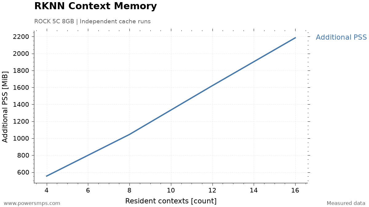
    In fresh standalone processes, allocating pools of 4, 8, 12, and 16 contexts yielded measured additional PSS memory footprints of 554.8 MiB (approx. 0.54 GiB), 1,046.1 MiB (approx. 1.02 GiB), 1,621.5 MiB (approx. 1.58 GiB), and 2,185.4 MiB (approx. 2.13 GiB), respectively.

    Measured additional PSS (MiB) scaling trend according to the number of resident RKNN contexts (4, 8, 12, 16) during standalone process execution on Radxa ROCK 5C 8GB.
    Measured additional PSS (MiB) scaling trend according to the number of resident RKNN contexts (4, 8, 12, 16) during standalone process execution on Radxa ROCK 5C 8GB.

    While additional PSS broadly exhibits an upward trend as contexts increase, the relationship is not strictly linear. Furthermore, this limited caching strategy loses practical utility due to the forward execution structure of the DiT.

    Sequential invocation sequence for step n (total 84 models)
    [Model 00 (self) → Model 01 (cross) → Model 02 (FFN) → ... → Model 83 (FFN)]
      ↓ Residual connection accumulation and scheduler latent update
    Sequential invocation sequence for step n+1 (identical pass across all 84 models)
    [Model 00 (self) → Model 01 (cross) → Model 02 (FFN) → ... → Model 83 (FFN)]
    

    Each branch output in a DiT block is immediately summed into the host’s FP32 residual stream and fed as input to subsequent branches and blocks. Furthermore, only after all 84 branch operations complete can the sampler update the denoising latent representation and advance to the next diffusion step. That is, loop interchange to reorder invocations is impossible due to sequential dependencies between models.

    Structurally, all 84 models are cyclically referenced in fixed order 1 times per 1 step. Before the same model can be re-invoked, 83 other models must be evaluated. Therefore, under any standard LRU cache with capacity strictly below 84 (e.g., capacity 4, 8, 16, 28, 56, etc.), every loaded model is inevitably evicted just before it could ever be reused: – LRU simulation result: across a total of 1,092 invocations, 0 hits / 1,092 misses (0% cache hit rate)

    Even if static pinning were applied to keep select models (e.g., model 0~15) in memory without eviction, the maximum time savable across 16 models amounts to only 16 model’s lifecycle per compute step. For 1 image, this reaches an absolute theoretical maximum savings of only approximately 72.4 seconds—which is not an empirically verified measurement. In return, the price paid is an additional PSS overhead of 2.13 GiB (2,185.4 MiB) and swap churn during sustained retention. Sacrificing system stability and inducing swap jitter for a modest theoretical saving of 72.4 seconds represents an unsound engineering trade-off.


    7. Configuration Maintained on 8GB

    The core bottlenecks and empirical findings derived from the W8A8 FFN integer quantization and resident context cache experiments are summarized below:

    • FFN W8A8 quantization: Computation accelerated, but fell short of visual quality standards.
    • Full model residency: Swap activity increased at 18 contexts, and additional PSS for 84 resident models extrapolated to approximately 11.3 GiB.
    • Limited caching: Under cyclic invocations, models were evicted before reuse, yielding zero LRU cache hits.

    On the ROCK 5C 8GB, we retained the FP16 models and chose an on-demand strategy: staging and executing each required model sequentially, followed immediately by release. In this comparison, the memory penalty far outweighed the latency benefits of keeping models resident.

    This decision applies specifically to this 8GB board and partitioned configuration. If memory capacity or model partitioning strategies change, the trade-offs of residency must be re-evaluated.

    Instead of stacking models in memory, can the graph partitioned into 84 subgraphs be consolidated into fewer models? In Part 4, we upgrade the compiler version to attempt graph operator fusion and compare latency and memory trade-offs.

  • RKNN Toolkit 2.3.2 vs 2.3.0: AdaLN Compiler Crash and Operator Fusion Benchmark

    RKNN Toolkit 2.3.2 vs 2.3.0: AdaLN Compiler Crash and Operator Fusion Benchmark

    Affiliate Disclosure: This post contains AliExpress affiliate links. If you make a purchase through these links, the author may receive a commission.


    1. Can Partitioned DiT Blocks Be Recombined?

    When deploying generative Diffusion Transformers (DiT) in embedded NPU environments, runtime memory limits and operator support constraints are critical factors directly dictating architectural design. This in-depth experiment was conducted on 2026-8-20 on a Radxa ROCK 5C 8GB single-board computer.

    The experiment used a directly purchased ROCK 5C 8GB board.

    The test board is a RK3588S2-based ROCK 5C, and the RKNN target is rk3588. It should be distinguished from the ROCK 5C Lite listed on the same product page.

    In Part 1, the Anima configuration partitioned the 28 DiT blocks into attention, cross-attention, and FFN components, yielding 84 FP16 RKNN models, with AdaLN and residual additions handled on the CPU. Here, we examined whether the 3 models per block could be fused into a single model.

    The baseline pipeline processed AdaLN (Adaptive LayerNorm) operations and residual additions in the host CPU Python runtime. However, repeatedly loading, executing, and releasing 3 subgraphs per step within a single DiT block—round-tripping intermediate tensors to the CPU host—incurs substantial driver overhead. If self-attention, cross-attention, FFN, and AdaLN within a block could be fused into a single RKNN graph (a fused 1-model), we expected to reduce the lifecycle invocations per block from 3 to 1 while eliminating host tensor transfer overhead.

    However, compiling a graph containing AdaLN operators under RKNN Toolkit 2.3.2—the default compiler at the time—triggered a fatal compiler segmentation fault (SIGSEGV, exit code 139). We first had to determine whether this crash stemmed from fundamental hardware non-support for the Anima DiT architecture or a compiler bug.


    2. Building the Same AdaLN Graph with Different Toolkits

    To isolate the compiler crash, we extracted a minimal ONNX reproducer containing only the crashing AdaLN operator instead of the full DiT block and ran compilation experiments.

    We compiled the identical AdaLN reproducer graph using RKNN Toolkit 2.3.2 and 2.3.0. All other build conditions were kept constant to compare results across compiler versions.

    Using the identical reproducer ONNX model, target (rk3588), and single-core optimization settings, the build results were as follows:

    Toolkit VersionAdaLN Graph BuildExit Code
    2.3.2Failed: SIGSEGV139
    2.3.0Success0

    In 2.3.2, the build aborted with a SIGSEGV immediately following LayerNorm graph optimization. In 2.3.0, the identical graph built without errors.

    Because the outcome differed solely by version on identical input graphs and targets, we determined this failure to be a compiler regression. The older 2.3.0 release provided a functional workaround for this graph, rather than resolving the issue by upgrading to a newer release.


    3. Verifying Fused Model Execution at 64px and 512px

    Using Toolkit 2.3.0, we compiled a fused model for the first DiT block and verified both a 64px test configuration and a 512px production inference configuration.

    Fused Block ResolutionRKNN ConversionOn-Board Execution
    64pxSuccessInit and inference verified
    512pxSuccessInit, inference, and release verified

    The 512px model build completed without triggering system swap. However, because certain Transpose and Erf operations were offloaded to the CPU, fusing into a single RKNN file does not mean every operator executes entirely on the NPU.

    A more critical validation checkpoint was binary compatibility with the target board’s local runtime. Even if compiled with 2.3.0, deployment complexity escalates sharply if the board OS’s RKNPU kernel driver or runtime libraries must be forcibly replaced.

    The compiled model was executed under runtime API 2.3.0 and driver 0.9.8. Without modifying the kernel or driver, we verified loading, initialization, inference, and context release across 3 repeated rounds of conditional and unconditional inference.

    In this single-block validation, switching only the compiler environment was sufficient to execute on the existing board runtime.


    4. Numerical Differences in Single-Block Output

    Once hardware execution of the fused model was verified, we performed a single-block correctness gate to confirm whether the NPU fused operation numerically matched the original floating-point reference tensors. The references used were the original PyTorch FP16 block outputs and ONNX Runtime (ORT) outputs.

    Target Architecture Reference Tensor Cosine Similarity Max Absolute Error (Max Abs) Mean Absolute Error (Mean Abs) Mean Squared Error (MSE) NaN/Inf Detection
    64px Fused PyTorch 0.99998315 0.28125 0.0018879 4.2748e-05 0 / 0
    64px Fused ONNX Runtime 0.99998608 0.28125 0.0018948 3.5387e-05 0 / 0
    512px Split (Baseline) PyTorch 0.99999881 0.14937 0.0002283 1.0841e-06 0 / 0
    512px Fused (Candidate) PyTorch 0.99997673 0.25000 0.0011279 2.1100e-05 0 / 0
    512px Fused (Candidate) ONNX Runtime 0.99997590 0.28906 0.0011662 2.1854e-05 0 / 0

    The 512px fused model recorded a cosine similarity of 0.99997673 and a maximum absolute error of 0.25000 against the PyTorch reference output, with no NaNs or Infs detected.

    However, the fused model’s MSE was 2.1100e-05, roughly 19.5 times higher than the 1.0841e-06 of the baseline split architecture. High cosine similarity on a single block alone cannot guarantee the image quality of the final output after traversing all 28 blocks over multiple steps.


    5. Fewer Context Invocations, but Only a 0.47% Speedup

    The primary motivation for pursuing subgraph fusion was latency reduction. We anticipated measurable speedups by migrating AdaLN and residual operations from host Python into the compiled graph, thereby reducing driver context invocations.

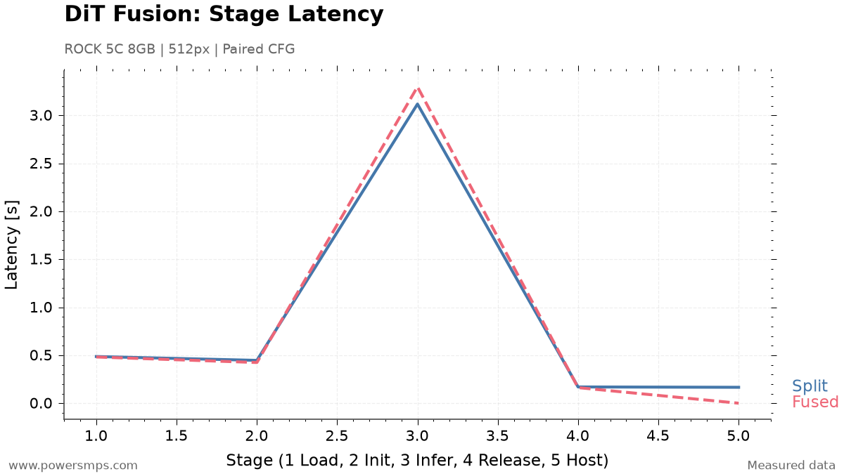
    On the ROCK 5C board, we executed 3 rounds of a 2-pass Classifier-Free Guidance (CFG) computation stream for a 512px single block and precisely measured the average execution time of each stage.

    512px DiT single-block measured component breakdown. 1=load, 2=init, 3=inference×2, 4=release, 5=host AdaLN/residual. Component total is Split 4.3856 s, Fused 4.3650 s.
    Comparison of component latency breakdown between Split 3-Model baseline and Fused 1-Model candidate for 512px single block on Radxa ROCK 5C.

    The table below compares measured latency stage-by-stage between the baseline 3-model split configuration and the candidate Fused 1-model configuration.

    Execution Stage & Component Baseline 3-Model Split Candidate Fused 1-Model Fused Delta Cause of Change & Analysis
    Model Load 0.4863 s 0.4814 s -0.0049 s Weight file loading time (marginal reduction for a single block)
    Runtime Init 0.4464 s 0.4240 s -0.0224 s Slight reduction in NPU runtime context initialization time
    NPU Inference (×2) 3.1177 s 3.2972 s +0.1795 s (+5.76%) NPU execution slowdown due to operator fusion
    Context Release 0.1694 s 0.1623 s -0.0071 s Context memory release time
    Host AdaLN & Residual 0.1658 s 0.0000 s -0.1658 s (-100%) Elimination of separate Python host AdaLN path
    Net Component Sum 4.3856 s 4.3650 s -0.0206 s (-0.47%) Actual net time saved was merely 0.0206 s
    Measured Wall Time 4.7379 s 4.4981 s -0.2398 s (-5.06%) Includes instrumentation distortion from multiple memory snapshots in split mode

    The benchmark data revealed bottlenecks that ran counter to intuitive expectations. First, host compute time of 0.1658 s was completely eliminated to 0 s in the Fused model. However, pure NPU forward inference time (Inference ×2) increased by +0.1795 s (+5.76%) from 3.1177 s to 3.2972 s. The increased inference latency in the fused configuration completely offset the savings gained by removing host compute (0.1658 s).

    Second, while context invocations dropped by 66.7% from 3 to 1, lifecycle overhead (Load, Init, Release) did not decrease as expected. Total single-block lifecycle time fell only by 3.1% from 1.1021 s to 1.0678 s. This revealed that practical RKNPU driver initialization and loading overhead is governed by total model file weight footprint (approximately 140~155 MB) and graph complexity rather than raw C API call counts.

    Third, while measured wall time appeared to decrease by 0.2398 s (5.06%), this figure included profiling overhead from collecting memory snapshots 6 times across 3 sub-contexts in split mode. Excluding snapshot measurement distortion, the actual net speedup based on pure component totals was merely 0.0206 s (-0.47%) per block.


    6. NPU Device Mapping Memory Increased by 94.30 MiB

    While the latency reduction was negligible, runtime memory suffered significant penalties. The memory metrics measured at the board level were as follows:

    Memory Metric Baseline 3-Model Split Candidate Fused 1-Model Difference & Rate of Change
    NPU Device-Mapped Device PSS 127,144 KiB 223,704 KiB +96,560 KiB (+94.30 MiB, +75.9%)
    Peak Process PSS During Execution 648,282 KiB 694,882 KiB +46,600 KiB (+45.51 MiB, +7.2%)
    New System Swap Generated 0 0 0 (Safe for single block)

    The split architecture executes each branch sequentially before releasing it. The peak NPU device mapping maintained at any one time was 127,144 KiB, or approximately 124.16 MiB.

    The fused architecture retains the entire block within a single runtime context. Device mapping increased to 223,704 KiB—approximately 218.46 MiB—consuming an additional 94.30 MiB.

    On the ROCK 5C sharing 8GB of total LPDDR4X memory—where the background OS, text encoder, and VAE must coexist—a 75.9% surge in device-mapped memory introduces severe system pressure.


    7. Why Operator Fusion Was Not Adopted

    Extrapolating single-block differences across the complete pipeline suggested an estimated reduction of approximately 7.51 s. This estimate was not measured by running full image generation.

    • Speed: Reductions in host compute were largely cancelled out by increased NPU inference latency.
    • Memory: Executing the same block required higher device-mapped memory.
    • Precision: Although single-block cosine similarity was high, MSE was larger than in the baseline split configuration.

    Because speedup was capped at 0.47% while memory consumption expanded, we retained the baseline split architecture for this board.

    The verification scope was limited to a single block. These findings do not reflect experiments fusing all 28 blocks to generate complete images or prolonged operational testing.

    Both the residency experiment in Part 3 and this fusion experiment demonstrated that reducing call counts alone cannot account for overall performance. NPU compute time and memory overhead must be evaluated together to choose optimizations viable on a 8GB board.

  • Generating Anima Images on RK3588: RKNN Conversion and Execution on ROCK 5C 8GB

    Generating Anima Images on RK3588: RKNN Conversion and Execution on ROCK 5C 8GB

    Affiliate Disclosure: This post contains AliExpress affiliate links. If you make a purchase through these links, the author may receive a commission.

    1. Running Anima on ROCK 5C 8GB

    With 8GB of memory, the Radxa ROCK 5C 8GB single-board computer (SBC) was used to verify on-device execution of a multi-billion-parameter Diffusion Transformer (DiT) model.

    The main processor of the board is a Rockchip RK3588S2 SoC, and its dedicated Rockchip NPU runtime target is rk3588. In the same manufacturer’s Radxa ROCK 5C product line, the Lite model with the RK3582 option uses a different chipset with scaled-down NPU units and CPU core configurations. Therefore, to reproduce this 8GB DiT compute pipeline, one must verify the RK3588S2-based ROCK 5C 8GB model.

    The DiT responsible for Anima’s image generation consists of 28 blocks. In this experiment, we partitioned and converted it into a format executable on the NPU of the ROCK 5C.

    The fixed I/O specifications for the on-device conversion are as follows: – Batch size: 1 – Generation resolution: 512×512 pixels – Input token specification: 1024 image tokens, 512 text conditioning tokens – Target ONNX version: Opset 19

    Qwen3 was used for text encoding, and Qwen-Image VAE was used for image reconstruction. In this configuration, the primary DiT compute is handled by the NPU, while text encoding and VAE decoding are handled by the CPU.


    2. Why the DiT Was Partitioned into 84 RKNN Models

    Packaging all 28 blocks of the DiT architecture into a single monolithic RKNN model ran into structural limitations of the RKNN compiler. In our 2026-8 experiments using the RKNN-Toolkit2 2.3.2 environment, compiling the entire DiT block or building branches combined with AdaLN (Adaptive Layer Normalization) operations caused a native segfault (exit 139).

    Decomposing the graph down to minimal units for debugging revealed that while large Linear layers or standard GELU FFN graphs compiled properly for the NPU target, subgraphs containing the AdaLN LayerNorm + broadcast shift/scale/gate pattern consistently triggered the same segfault regardless of weight size. This confirmed that the issue was not out-of-memory, but a compiler error in parsing specific graph operator patterns.

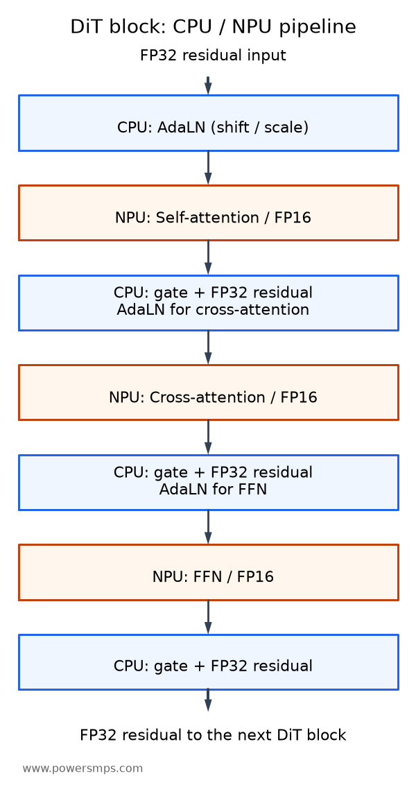
    We separated the 3 compute branches that can execute on the NPU in each DiT block, handling normalization, gating, and residual summation on the CPU.

    Each of the 28 DiT blocks was divided into 3 subgraphs: self-attention, cross-attention, and FFN. Self-attention computes relationships between image tokens, cross-attention computes relationships between text conditioning and image tokens, and FFN transforms the features of each token.

    DiT block architecture alternating between blue CPU stages and orange NPU stages. The CPU handles AdaLN, gate multiplications, and FP32 residual accumulation for each branch, while the NPU processes FP16 self-attention, cross-attention, and FFN.
    CPU/NPU execution sequence for a single DiT block. The NPU processes FP16 attention and FFN, while the CPU handles AdaLN before each branch, gate multiplications after each branch, and FP32 residual accumulation. This structure repeats across 28 blocks.

    A total of 84 (28 × 3) FP16 RKNN models were generated, totaling approximately 3.99GB in size. AdaLN, gate multiplication, RoPE, input/timestep embeddings, and final projection were executed on the CPU. Residual accumulation was maintained in FP32.

    • Separate operations to be handled by the CPU from operations to be handled by the NPU in the original model.
    • Convert NPU operations into fixed-I/O-shape ONNX graphs and then compile them to RKNN.
    • Compare single-block and full-block outputs against the original model before running image generation.

    3. How Close Are the Outputs Before and After Conversion

    The most critical step in hybrid partitioned conversion is preventing numerical error accumulation across frameworks. We separated verification into single-block validation and sequential cumulative validation across all 28 blocks.

    Single-Block Comparison

    We compared ONNX and RKNN outputs against the original PyTorch block’s FP16 branch operations and FP32 residual accumulation. This step verifies whether the converted operations produce outputs pointing in the same direction as the original model.

    Comparison Target Cosine Similarity (Cosine) Mean Absolute Error (MAE) Maximum Absolute Error (Max AE) NaN / Inf Occurrences
    PyTorch → ONNX 0.9999994183 0.00012350 0.09396 0 / 0
    PyTorch → RKNN 0.9999990896 0.00019535 0.11446 0 / 0
    ONNX → RKNN 0.9999995474 0.00014175 0.06969 0 / 0

    The cosine similarity between the baseline PyTorch output and the RKNN output was 0.9999990896. For a single block, the outputs before and after conversion maintained highly aligned trajectories.

    Output Comparison Across 28 Blocks

    To confirm that numerical errors do not amplify while passing from Block 0 through Block 27 across all 28 blocks, we compared the pure ONNX accumulated tensor against the RKNN 84-core accumulated tensor.

    • Lowest single-block cosine similarity: 0.999993668 (lowest among all 28 blocks)
    • Final hidden layer similarity (Hidden Cosine): 0.9999989412
    • Final 16-channel prediction tensor similarity (Final Prediction Cosine): 0.9999989072
    • Final prediction tensor MAE: 0.00129712
    • Final prediction tensor Max AE: 0.00830078
    • Boundary NaN / Inf occurrences: 0

    Even after passing through 28 blocks, no NaNs or Infs occurred, and high similarity to the reference output was preserved. However, this numerical comparison must be distinguished from the perceptual quality evaluation of the final generated image.


    4. How Long Did Denoising Take?

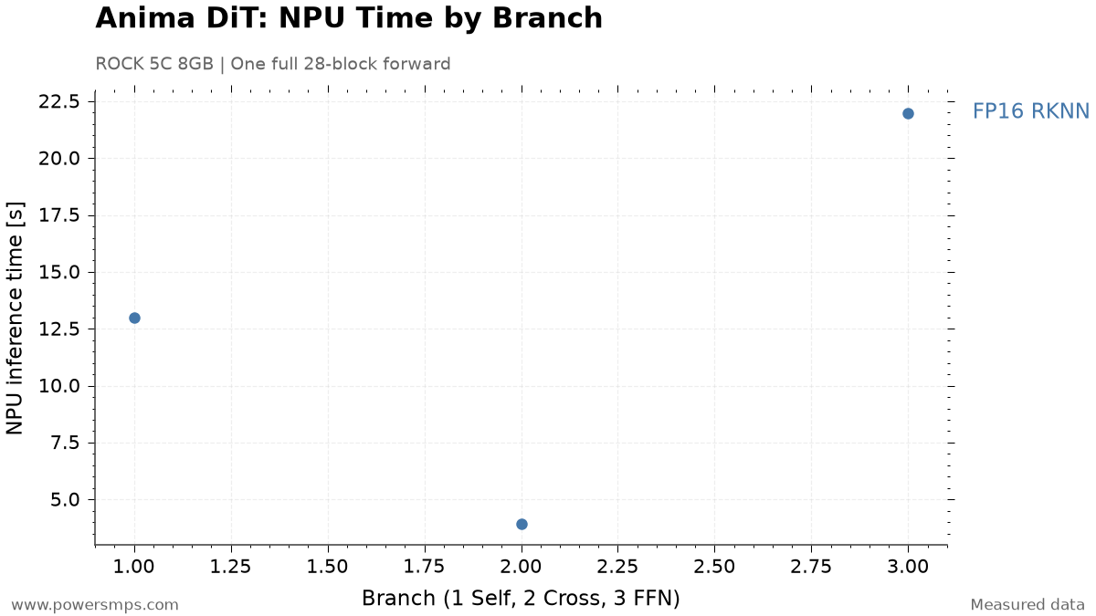
    Pure NPU Latency by Branch Across Full 28-Block Forward Pass

    On the RK3588 NPU, the total pure inference time for a single forward pass through all 28 DiT blocks is approximately 38.90 seconds. The branch-by-branch values below represent the summed execution times across all 28 blocks.

    The detailed latency breakdown by core is as follows: – Self-Attention Core: 12.99 seconds – Cross-Attention Core: 3.92 seconds – FFN Core: 21.99 seconds

    NPU inference time sum by branch in a single full DiT forward pass on the ROCK 5C across all 28 blocks. 1: self-attention, 2: cross-attention, 3: FFN. Not single-block latency.
    NPU inference time sum by branch in a single full DiT forward pass on the ROCK 5C across all 28 blocks. 1: self-attention, 2: cross-attention, 3: FFN. Not single-block latency.

    The parameter-heavy FFN core accounts for approximately 56.5% of total pure NPU inference time. Note that the total wall-clock time for the full 28-block test accompanied by ONNX numerical validation logic was 162.8 seconds, which is distinct from the pure NPU compute time (38.90 seconds).

    20-Step Sequential CFG Denoising Results

    We executed the actual image generation workflow—a 20-step sequential Classifier-Free Guidance (CFG, guidance scale 4.0) denoising process—directly on the board. Due to memory constraints, conditional (positive) and unconditional (negative) predictions were not batched together, but processed via sequential invocations.

    • 20-step denoising: 2,408.54 seconds
    • Per-step average: 120.40 seconds
    • Pure NPU compute per step: 76.21 seconds
    • Model staging, host processing, etc. per step: approx. 44.19 seconds
    • NaN/Inf occurrences across all 20 steps: 0

    The approximately 44.19 seconds of non-NPU overhead per step includes loading, initialization, and releasing (load/init/release) across the 84 RKNN models, as well as host computation and boundary marshalling costs. Subsequent optimizations will isolate and profile these components individually.


    5. Reducing Image Reconstruction Time by Replacing the VAE

    The VAE decoding process, which reconstructs the denoised latent representation into a 512×512 pixel RGB image, poses a heavy CPU compute burden. Using the official Diffusers Qwen-Image VAE FP32 CPU implementation as-is resulted in a decoding latency of 2,154.51 seconds (approx. 35 minutes 54 seconds), introducing a severe bottleneck on par with the total 20-step DiT denoising time.

    For VAE decoding, we applied an ARM NEON- and OpenMP-optimized CPU implementation from stable-diffusion.cpp. Rather than re-initializing the text encoder and transformer, the pipeline was linked to receive only the post-denoised latent tensor and reconstruct the image.

    Configured with 4 CPU threads, a tile size of 32×32, and an overlap of 0.5, the comparison results between VAE backends are as follows:

    Metric Official Diffusers FP32 VAE sd-cpp Tiled CPU VAE Improvement
    Decoding Latency 2,154.51 seconds 155.04 seconds 13.90× faster (1,999.47 seconds saved)
    PSNR (vs. Diffusers Output) Baseline 31.444 dB Compared to reference
    11×11 Gaussian SSIM 1.00000 0.96109 Compared to reference
    Output Resolution & Format 512×512 RGB 512×512 RGB NaN / Inf: 0

    Visual inspection confirmed that composition, color, and fine details were well preserved. While PSNR and SSIM do not imply identical outputs, decoding time was reduced to the 2 minutes 35 seconds range.

    Total Latency: Denoising Plus Image Reconstruction

    Integrating VAE acceleration yields the following overall image generation latency: – DiT 20-step sequential CFG denoising: 2,408.54 seconds – sd-cpp tiled VAE decoding: 155.04 seconds – Total generation time (excluding 1-time prompt encoding): 2,563.58 seconds (approx. 42 minutes 44 seconds)


    6. The Next Bottleneck: Denoising

    By reducing VAE decoding latency from 2,154.51 seconds to 155.04 seconds, the VAE’s share of overall pipeline latency dropped dramatically from 47.2% to 6.0%. Consequently, the dominant system bottleneck shifted to DiT 20-step denoising (2,408.54 seconds, 94.0% of the total).

    Deconstructing DiT denoising internally shows that pure NPU compute takes 76.21 seconds per step (across 20 steps, totaling 1,524.20 seconds), while the remaining approximately 884.34 seconds consists of non-NPU overhead including model lifecycle and host processing. Context residency was considered as a candidate to eliminate repetitive initialization costs, but memory headroom and actual savings required independent verification under an 8GB environment. Those experimental results are covered in Part 3.

    Subsequent optimizations examined compute iteration count alongside memory usage. Part 2 covers reducing compute steps with Spectrum, while Part 3 explores the limits of quantization and model residency against image quality and memory constraints. In Part 4, we evaluate compiler version differences and the trade-offs of graph operator fusion.