Author: mk

  • 220Vac SMPS Input Smoothing Capacitor Sizing: Calculation and Simulation Example

    220Vac SMPS Input Smoothing Capacitor Sizing: Calculation and Simulation Example

    For smoothing capacitors, after calculating capacitance from the allowable ripple, tolerance and minimum bus voltage must be verified. Taking a 60W SMPS with bridge-rectified 220Vac as an example, this article walks through the calculation and examines ripple and charging current using rectified waveforms.

    The previous article ‘How to Select a Smoothing Capacitor’ covered voltage ratings and selection principles using Schade curves. Here, the initial capacitance is determined using the energy equation for a constant-power load. The numerical values are based on the conditions of the design example.

    1. Design Conditions: 220Vac, 60W, Ripple 40Vpp

    The target circuit consists of a single-phase bridge rectifier without PFC and an input bulk capacitor. The connection sequence is AC source → source resistance → bridge rectifier → bulk capacitor and DC/DC input load. The capacitor’s ESR is included in series, and the bus DC return is separated from protective earth. Because this calculation example deals with a high-voltage non-isolated section directly connected to utility power, it is structured as an example for circuit operation verification and numerical analysis.

    Parameter Example Condition
    Rated Input and Variation 220Vac ±10%, i.e., 198~242Vac
    Line Frequency 50/60Hz, capacitance calculation based on 50Hz
    DC/DC Output Power 60W
    DC/DC Stage Efficiency Assumed to be 85%
    Allowable Bus Ripple 40Vpp
    Capacitor Initial Capacitance Tolerance −20%
    Bridge Voltage Drop for Calculation Sum of two conducting diodes 2V

    The 220Vac case serves as an appropriate baseline to explain the operation of line-operated SMPS. However, 85~264Vac universal input or PFC buses operate in different operating regimes and require separate calculations. The allowable ripple of 40Vpp is the target value for this design, and whether the downstream DC/DC can operate stably even at the ripple valley must be verified against the actual converter’s input range.

    2. Constant-Power Loads Are Calculated Using Energy Equations

    Assuming the DC/DC maintains output power, the average power drawn from the bus is as follows. Here, 85% is the efficiency assumed to evaluate the conversion power of the DC/DC stage, excluding losses in the bridge and input stage.

    \[ P_{\mathrm{bus}}=\frac{P_{\mathrm{out}}}{\eta_{\mathrm{DC/DC}}} =\frac{60}{0.85}\approx70.59\,\mathrm{W} \]

    Because the bus current is \(I=P_{\mathrm{bus}}/V_{\mathrm{bus}}\), it increases as the voltage drops during discharge. Therefore, rather than fixing a single current value in \(C=I\Delta t/\Delta V\) assuming a constant current, it is more appropriate to use the capacitor’s energy change.

    \[ P_{\mathrm{bus}}\Delta t=\frac{1}{2}C_{\mathrm{eff}} \left(V_{\mathrm{hi}}^2-V_{\mathrm{lo}}^2\right),\qquad C_{\mathrm{eff}}=\frac{2P_{\mathrm{bus}}\Delta t}{V_{\mathrm{hi}}^2-V_{\mathrm{lo}}^2} \]

    The ripple frequency of full-wave rectification is twice the line frequency. First, neglecting the charging time, the discharge time is taken as \(\Delta t\approx1/(2f_{\mathrm{line}})\), which is 10ms at 50Hz. This is a conservative 1st-order approximation with a longer discharge time to quickly estimate the initial capacitance. Appendix A of Power Integrations AN-92 also calculates the bulk capacitor from the energy balance of a constant-power load while the rectifier is blocked.

    At the low line input of 198Vac, the calculated charging peak and target minimum voltage are as follows.

    \[ V_{\mathrm{hi}}\approx198\sqrt{2}-2=278.01\,\mathrm{V},\qquad V_{\mathrm{lo}}=278.01-40=238.01\,\mathrm{V} \]

    \[ C_{\mathrm{eff,min}}\approx \frac{2\times70.59\times0.010}{278.01^2-238.01^2} \approx68.4\,\mu\mathrm{F} \]

    Applying an initial tolerance of −20%, a nominal capacitance of \(C_{\mathrm{nom}}\ge68.4/0.8\approx85.5\,\mu\mathrm{F}\) is required. Therefore, 100µF is selected as the initial candidate. Here, the initial tolerance is applied to establish a 1st candidate; in an actual design, the final margin is confirmed by also accounting for capacitance variation over temperature and operating lifetime.

    3. Compare Candidate Capacitances Using Minimum Effective Values

    Ripple can be recalculated and compared using the equation below. The effective capacitance in the comparison table is 80% of the nominal value, and the same low-line peak of 278.01V is used in the approximate calculation.

    \[ V_{\mathrm{lo}}\approx\sqrt{V_{\mathrm{hi}}^2- \frac{2P_{\mathrm{bus}}}{2f_{\mathrm{line}}C_{\mathrm{eff}}}},\qquad \Delta V_{\mathrm{pp}}=V_{\mathrm{hi}}-V_{\mathrm{lo}} \]

    Nominal Capacitance −20% Effective Capacitance 50Hz Approximate Ripple 60Hz Approximate Ripple 50Hz Simulated Ripple
    68µF 54.4µF 51.4Vpp 42.1Vpp 40.4Vpp
    82µF 65.6µF 41.9Vpp 34.4Vpp 33.7Vpp
    100µF 80µF 33.8Vpp 27.8Vpp 27.8Vpp
    120µF 96µF 27.8Vpp 23.0Vpp 23.2Vpp

    Under the approximation criteria, 82µF exceeds the 50Hz·40Vpp target, whereas 100µF satisfies it. Applying the effective capacitance of 80µF for the 100µF candidate yields an approximate 50Hz ripple of about 33.8Vpp and a minimum voltage of about 244.2V. At 60Hz, the recharge interval becomes shorter, reducing the ripple. The simulated values in the table reflect the circuit conditions described in the next section.

    4. How Much Do Circuit Waveforms Differ from Calculated Values?
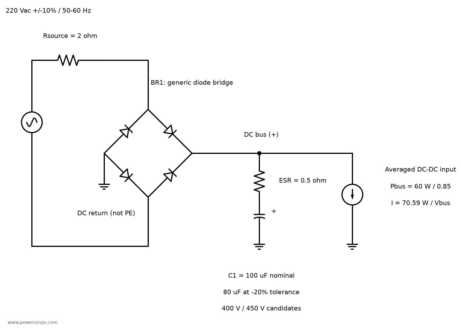
    220Vac bridge rectifier, source resistance, smoothing capacitor with series ESR, and constant-power DC/DC input load
    Bridge rectifier and smoothing circuit for 220Vac input. The DC return is separated from protective earth.

    The waveforms below show transient simulation results of the bridge rectifier circuit performed in ngspice. The input source resistance is assumed to be 2Ω, and the capacitor ESR is assumed to be 0.5Ω. All four diodes use the same generic model. The model parameters are IS=5nA, N=1.8, RS=0.1Ω, BV=1000V, and IBV=10µA. Rather than being restricted to specific commercial components, the modeling is intended to verify fundamental circuit behavior.

    The load is an averaged constant-power model with \(I_{\mathrm{load}}=70.59/V_{\mathrm{bus}}\). To ensure startup calculation stability, the denominator was clamped below 200V, and the load was ramped up gradually over 50~55ms. The results were evaluated during the steady state at 0.5~0.6 seconds. In this interval, it was verified that the bus remains above 200V and load power maintains its setpoint. The maximum simulation timestep is 20µs. Behavioral sources and transient analysis methods can be referenced in the ngspice manual.

    198Vac · 50Hz · Effective 80µF Parameter Simulation Result
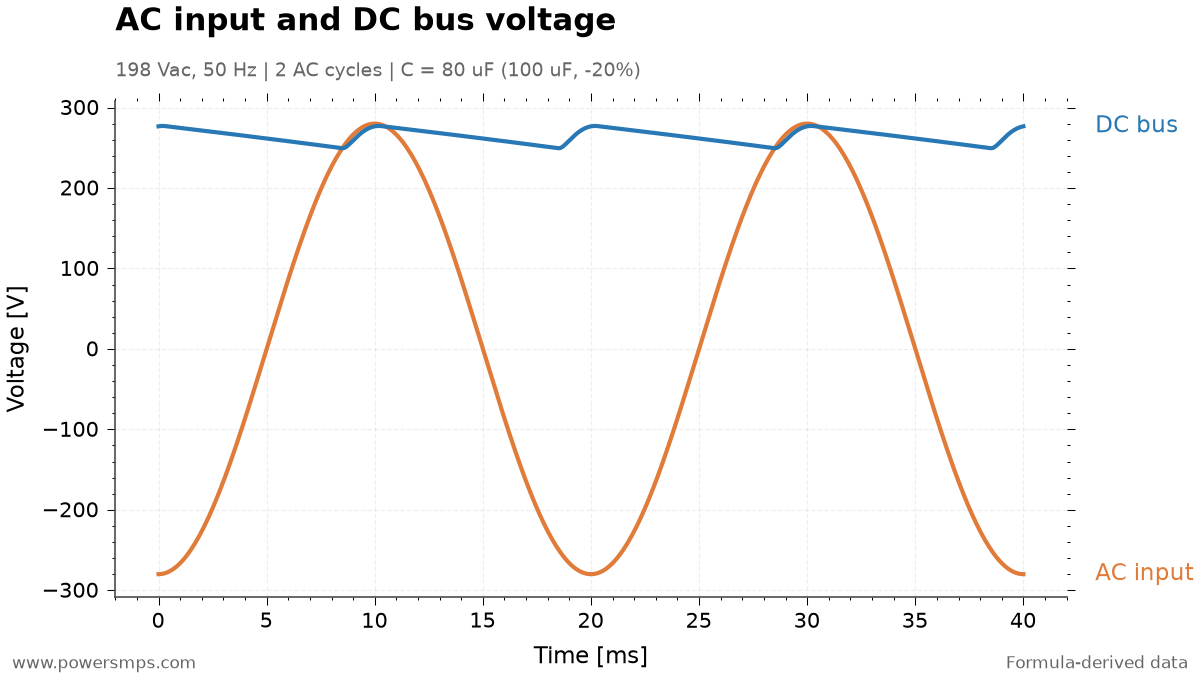
    Maximum Bus Voltage Approx. 277.1V
    Minimum Bus Voltage Approx. 249.3V
    Bus Ripple Approx. 27.8Vpp
    Capacitor Low-Frequency Ripple Current Approx. 0.654Arms
    Bridge Output Peak Charging Current Approx. 2.43A
    Input AC voltage and bus voltage plotted on the same voltage axis. 2 cycles (40ms) of 50Hz input AC, effective capacitance 80µF.
    Input AC voltage and bus voltage plotted on the same voltage axis. 2 cycles (40ms) of 50Hz input AC, effective capacitance 80µF.

    The simulated circuit value of 27.8Vpp is smaller than the simple calculated value of 33.8Vpp. This occurs because the rectifier conducts for a finite interval to supply the load and charge the capacitor, resulting in a shorter discharge duration than the calculation that assumes discharge over the entire half-cycle. Conversely, source resistance and diode forward drops reduce the achievable peak voltage. ST AN1262 also takes rectifier conduction time into account when evaluating input bulk capacitance and minimum bus voltage.

    Even if the 82µF candidate falls within 40Vpp in circuit simulation, adopting it immediately is premature. The resistance and diode parameters here are assumed values. It is safer to select the initial candidate using a conservative 1st-order calculation and then refine it using models and measurements reflecting actual components and operating conditions.
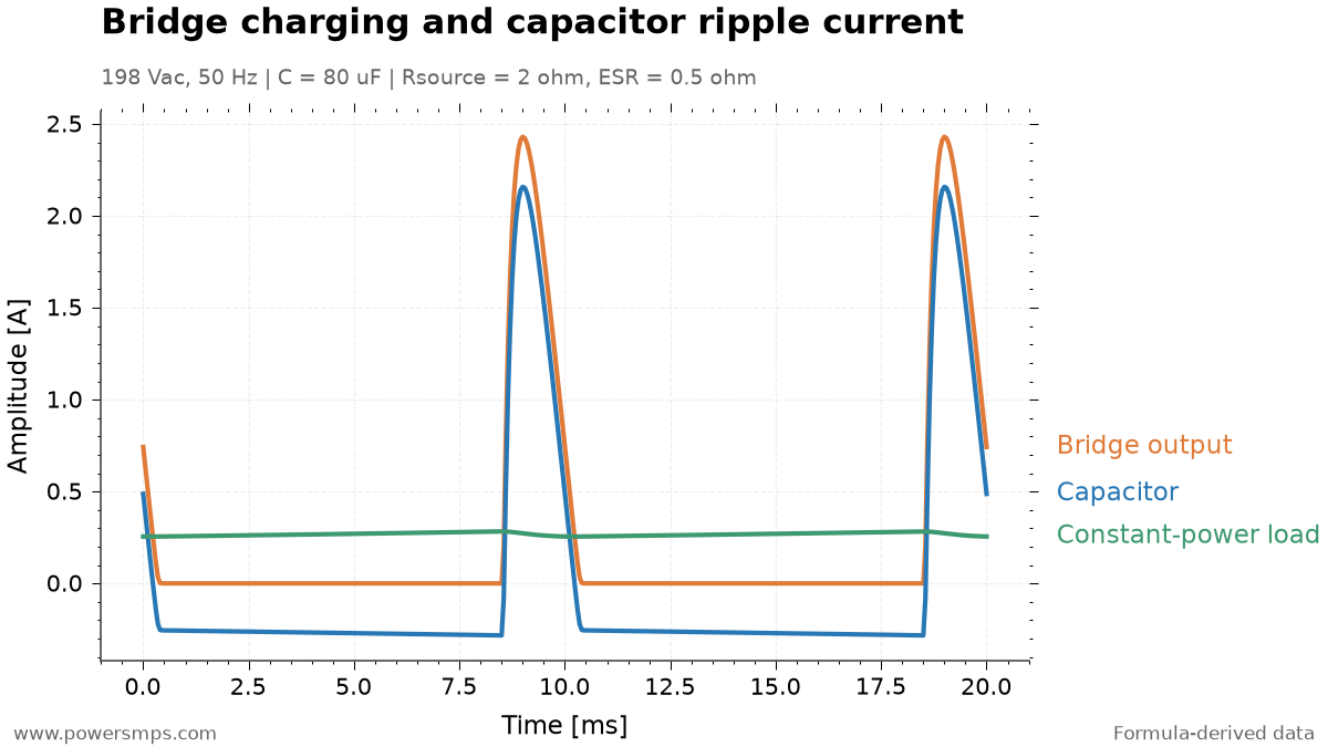
    Bridge output current, capacitor current, and load current. Positive capacitor current represents charging, negative represents discharging, and high-frequency switching currents are not included.
    Bridge output current, capacitor current, and load current. Positive capacitor current represents charging, negative represents discharging, and high-frequency switching currents are not included.

    The capacitor current is \(i_C=i_{\mathrm{bridge}}-i_{\mathrm{load}}\). It delivers current to the load during discharge and receives pulsating currents during charging. Therefore, allowable ripple current for the capacitor cannot be evaluated solely from the load current. The RMS value above represents the low-frequency component calculated as \(I_{C,\mathrm{rms}}=\sqrt{(1/T)\int i_C^2dt}\). The averaged load model does not include the high-frequency switching current of the DC/DC converter.

    5. Voltage Rating and Ripple Current Are Verified Separately

    At the high line input of 242Vac, the no-load peak calculated without diode forward drop is \(V_{\mathrm{pk,max}}\approx242\sqrt{2}=342.2\,\mathrm{V}\). Based on this steady-state voltage, 400V and 450V ratings can be compared as candidates. When determining the actual voltage rating, surge margins, voltage derating guidelines, and operating temperature must be comprehensively evaluated in addition to the steady-state peak.

    Ripple current ratings must be compared against the datasheet frequency and temperature specifications. A simple calculation of only the low-frequency ESR loss in this model gives \(P_{\mathrm{ESR}}\approx0.654^2\times0.5\approx0.214\,\mathrm{W}\). Actual dissipation must also account for frequency-dependent ESR and high-frequency current components. Temperature and lifetime considerations can be explored further in the article on smoothing capacitor lifetime, thermal management, layout, and venting. When increasing capacitance, startup inrush current and rectifier stress must also be verified.

    The ripple target must also be distinguished from holdup time. The 10ms in this 50Hz calculation is the periodic interval between rectification peaks. This differs from the requirement of maintaining output for 20ms following an AC line dropout. Holdup is evaluated separately using \(t_{\mathrm{hold}}\approx C_{\mathrm{eff}}(V_{\mathrm{start}}^2-V_{\mathrm{stop}}^2)/(2P_{\mathrm{bus}})\), which must incorporate the case where power drops out at the worst-case ripple valley and the downstream converter’s actual minimum operating voltage.

    6. Selection Results for This Example

    Under the conditions of 220Vac ±10%, 60W, DC/DC efficiency of 85%, 50/60Hz, and allowable ripple of 40Vpp, 100µF can be selected as the initial capacitance candidate. With an effective capacitance of 80µF reflecting the −20% tolerance, the approximate 50Hz ripple is about 33.8Vpp, and the circuit simulation value is about 27.8Vpp.

    After determining the 1st candidate capacitance by calculation, the criteria to check when finalizing component selection are as follows.

    • Verify that at low line (198Vac), the ripple valley remains above the minimum input voltage of the downstream DC/DC converter.
    • Determine a voltage rating (400V or 450V) that satisfies surge margins and derating standards based on the high line (242Vac) no-load peak voltage (342.2V).
    • Check whether temperature rise due to low-frequency ripple and high-frequency switching components, as well as startup inrush current, can be tolerated.
  • 74HC595 1-Bit Output Shift Issue: Burst Noise and CLK RC Filter Case Study

    74HC595 1-Bit Output Shift Issue: Burst Noise and CLK RC Filter Case Study

    I once used a 74595-series shift register to expand limited MCU output ports. However, during testing where a 1 kV burst was applied to the AC power port in accordance with EN 55014-2, an issue occurred where the output data shifted by 1 bit.

    Replacing the part with the TI SN74HCS595 featuring Schmitt-trigger inputs reduced the malfunction frequency, but the symptom persisted. While retaining the SN74HCS595, after adding an RC filter with a 100 Ω series resistor and a 1 nF capacitor to the CLK path, the phenomenon no longer occurred under the test conditions. This article summarizes the filter arrangement and troubleshooting process when distributing CLK to multiple ICs.

    Why False CLK Detection Causes Output Bit Shifts

    The 74595 architecture separates the shift register from the output storage register. In the case of the SN74HCS595, serial input data is shifted on the rising edge of SRCLK, and a separate RCLK updates the output storage register. This operational structure can be confirmed in the TI SN74HCS595 datasheet.

    If an unintended CLK edge is falsely detected during shifting, the data can shift by an extra bit. When RCLK subsequently updates the outputs, the shifted data appears on the parallel outputs.

    Based on the symptom of the output shifting by 1 bit and the improvement achieved after applying the CLK filter, we determined that this issue was caused by burst noise coupling into the shift CLK trace and being falsely recognized as additional clock pulses.

    Switching to the SN74HCS595: Frequency Reduced, but Symptom Persisted

    First, we replaced the IC with the TI SN74HCS595, which has Schmitt-trigger inputs. This device incorporates Schmitt-trigger architecture on all inputs, accommodating slow or noisy input signals. TI Datasheet

    A Schmitt trigger uses different switching thresholds for rising and falling input voltages. This hysteresis reduces repeated switching caused by chatter near the input threshold. However, if noise swings across both switching thresholds, even a Schmitt-trigger input can register it as a clock pulse.

    In practice, after replacing the IC, the malfunction frequency decreased, but the bit-shift issue did not disappear entirely. Because input hysteresis alone was insufficient in this environment, we added a countermeasure to attenuate the noise reaching the CLK input.

    Adding a 100 Ω and 1 nF RC Filter to CLK

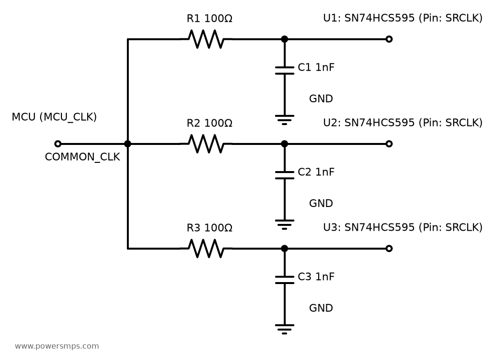
    While retaining the SN74HCS595, we inserted a 100 Ω resistor in series with the CLK signal path and connected a 1 nF capacitor between GND and the SRCLK input node downstream of the resistor.

    When distributing a common CLK to multiple ICs via stub traces, applying filters individually close to the CLK input of each IC proved effective. Because noise can also couple into traces downstream of the branch point, filtering at each receiving end is essential.

    Schematic diagram showing a 100 Ω series resistor and a 1 nF capacitor between the SRCLK input and GND applied to each branch of the common MCU CLK
    CLK branch 100 Ω series resistor and 1 nF filter between input and GND. The three branches represent an example configuration; DATA (SER), output latch (RCLK), power, and decoupling connections are omitted.

    The schematic is a conceptual diagram illustrating the filter connections for each branch. The three branches represent an example configuration; DATA (SER), output latch (RCLK), power, and decoupling connections are omitted.

    The connection sequence for each branch is Common CLK → 100 Ω series resistor → SRCLK input. The 1 nF capacitor connects from the input node downstream of the resistor to the local IC GND. Traces between the capacitor and GND should also be kept short.

    The RC filter dampens voltage swings at the input node in response to short noise pulses, while the Schmitt trigger evaluates the filtered input signal against its hysteresis thresholds. The two countermeasures serve complementary roles.

    Burst Test Results by Countermeasure

    Implementation Stage Observed Result
    Existing 74595-series IC used Output data shifted by 1 bit during burst testing
    Replaced with SN74HCS595 Malfunction frequency reduced, but bit-shift symptom persisted
    Retained SN74HCS595 + added 100 Ω / 1 nF RC filter to CLK No bit-shift issues observed under test conditions

    The above results were verified under test conditions where a 1 kV burst was applied to the AC power port in accordance with EN 55014-2. In this circuit, the symptom that remained after swapping the IC was resolved by adding the RC filter.

    Timing Considerations When Applying to Other Circuits

    The ideal RC time constant for 100 Ω and 1 nF is 100 ns. Although these component values resolved the issue in this circuit, the filter impacts not only noise but also the transition edges and arrival times of the valid CLK signal. Therefore, when adapting this solution to other circuits, the following items must be verified.

    • Valid CLK pulse width and input transition time: Verify that required clock conditions are still satisfied after filtering.
    • Data and output latch timing: Check the setup and hold times for SER, as well as the timing margin from the final SRCLK to RCLK, against datasheet specifications.
    • CLK arrival skew between multiple ICs: Account for skew caused by individual RC component tolerances and input threshold variations. In serial cascaded configurations in particular, verify data setup and hold margins between ICs.
    • MCU CLK output drive loading: As the number of branches increases, the cumulative capacitive load rises; review GPIO drive capability and actual signal transmission requirements.
  • RK3688 Release Status and Comparison Preparation: Performance and Thermal Baselines from ROCK 5C Measurements

    RK3688 Release Status and Comparison Preparation: Performance and Thermal Baselines from ROCK 5C Measurements

    Why I Am Preparing for the RK3688 Comparison

    The reason for waiting for the RK3688 is simple. I want to see how much faster image generation—which took a long time on the ROCK 5C—will become on the new board. While looking into the chip news, I also revisited the empirical measurement records I had accumulated.

    As of 2026-10-27, I am planning to purchase RK3688 hardware. Using the records from directly running the ROCK 5C as a starting point, I organized the items I want to compare once the new equipment arrives.

    When Will RK3688 Be Available?

    Following recent updates, what caught my attention was the product sequence. Looking at Rockchip’s disclosures alongside Radxa’s materials outlines which boards will arrive first and which will require waiting a bit longer.

    In the Rockchip 2026 Q3 Quarterly Report, Rockchip explained that RK3668 will enter production soon, followed subsequently by RK3688. This indicates that RK3668 will appear on the market ahead of the RK3688 I am waiting for.

    Also interesting from the Radxa official download server rock6/6b directory is the Rockchip RK3668 SoC Application REL02. In this 2026-10-09 page document, the RK3668 CPU is listed as consisting of 6 Cortex-A725 cores and 2 Cortex-A520 cores, with an NPU rated at 44 TOPS Sparse, and engineering samples slated for 2027 Q1.

    In particular, it is noteworthy that the document is hosted in the rock6/6b directory. Personally, I look forward to seeing what chip and memory configurations will appear in the ROCK 6 series. It would be even more welcome if the options extend from SBCs to highly expandable boards.

    Rockchip also introduced the RK3668 and RK3688 as its next high-performance platforms in the Rockchip official high-performance SoC roadmap announcement. I am keenly watching to see what kind of upgrade path these two chips will offer for those using the RK3588 series.

    Looking at the schedule, the picture I anticipate is that boards based on the RK3668 will arrive first, followed by RK3688 boards. Personally, rather than chasing immediate sale dates, I place more weight on watching whether boards that can actually be purchased become available next year. Along with release news, I am also looking forward to the SDK and memory configurations.

    RK3588 vs. RK3688: How Much Faster Will It Be?

    Comparing RK3588 and RK3688 on Paper

    First, I summarized the performance differences I am anticipating. The RK3688 specifications are planned figures based on the specification slides revealed at the 2025 Rockchip Developer Conference. Placing them side by side with the RK3588S2 configuration of the ROCK 5C I currently use makes it clearer why I look forward to this upgrade.

    ItemCurrent RK3588 Series / ROCK 5CRK3688 Published PlanAnticipated Change
    CPU Configuration4×Cortex-A76 + 4×Cortex-A55, 8 Cores8×Cortex-A730 + 4×Cortex-A530, 12 Cores1.5× total cores and 2× big cores for parallel workload headroom
    CPU Integer ThroughputReference value of 93K DMIPS from materials300K DMIPS or higherThroughput roughly 3.2× relative to the reference value
    NPU6 TOPS (INT8)RKNN-P3, 32 TOPS or higherNominal peak compute roughly 5.3×, expecting real-world model acceleration
    GPUMali-G610 MC4Mali-Magni, 2.0 TFLOPS or higherAnticipated increase in graphics and GPU compute headroom
    MemoryMy board: 8GB LPDDR4xLPDDR5/5x/6, planned up to 200GB/sAnticipating relief for large model loading and data transfers

    The CPU undergoes major changes not only in core count but also across architecture generations. Comparing the reference 93K DMIPS of the RK3588 with the planned 300K DMIPS for the RK3688 yields roughly 3.2×. I expect this difference will be particularly welcome during CPU preprocessing, postprocessing, and concurrent multitasking. Whether single-thread speed or VAE time scales by the same multiple will need to be observed separately under real workloads.

    The NPU increase from 6 to 32 TOPS is roughly 5.3×. Looking at the numbers alone, this is the most anticipated aspect, but the Anima pipeline I use mixes FP16 DiT execution with CPU processing. Therefore, in the time projections below, instead of directly applying the INT8 TOPS multiple, I separately assumed how much faster the entire denoising stage—including data movement and CPU processing—would become. For the GPU, I am looking forward to the architectural generation shift and the target of over 2.0 TFLOPS.

    Memory is another key motivation for upgrading. Moving from the current 8GB LPDDR4x environment to a board with faster memory and ample capacity should make model loading and repeated runs noticeably smoother. Because the maximum of 200GB/s is a chip design target from reference materials, I also intend to examine the actual memory configuration of the board I purchase closely.

    Empirical Usage Records Accumulated on the Current Board

    The baseline for comparison is the ROCK 5C 8GB that I operated. While waiting for the new board, I first reexamined where the existing environment spent its time and how warm it became.

    The board I used is the RK3588S2 model, the standard edition in the Radxa official ROCK 5C documentation, equipped with 8GB of memory. In software, the runtime target is specified as rk3588. Because the Lite model uses the RK3582, I recorded both the board name and chip name.

    The workload used for measurements is the 512×512 Anima image generation covered earlier in RKNN Conversion and Execution Results on ROCK 5C 8GB. The NPU and CPU divide the tasks as follows:

    Pipeline StageProcessing UnitRole
    Text EncodingCPUPrompt context generation
    DiT Attention / FFNNPUExecution of partitioned FP16 RKNN graphs
    Normalization, Gating, and Residual ProcessingCPUHost operations and FP32 residual accumulation
    VAE DecodingCPUReconstruction of latent representations into final images

    A comprehensive recount of raw job logs collected from 2026-8-13 to 8-25 shows that out of 649 total generation attempts, 404 completed successfully and 245 failed. The detailed duration distribution for the 404 successfully completed jobs is as follows:

    • Mean elapsed time: 1658.52 s (approx. 27.64 min)
    • Median: 1627.29 s (approx. 27.12 min)
    • Minimum elapsed time: 1513.56 s (approx. 25.23 min)
    • Maximum elapsed time: 1911.67 s (approx. 31.86 min)
    • 95th percentile (p95): 1799.59 s (approx. 29.99 min)

    Among the 404 completed runs, 20 tasks (approximately 4.95%) exceeded 30 minutes. Because these records date from a period of switching between various step configurations, an average of 27.64 minutes per image reflects my typical operating speed at the time. On the RK3688, I want to see how much the waiting time decreases when matching the same step count. With logs of the 245 failed attempts also preserved, I plan to examine both completion times and failure modes together on the new hardware.

    Temperatures and NPU Clocks Across 7002 Sensor Readings

    Along with speed, the other metric I revisited was temperature. Aggregating 7002 sensor samples collected at approximately 1-minute intervals from 2026-8-20 to 8-25 revealed thermal shifts across each zone of the board quite distinctly.

    Key statistics across thermal sensor zones observed across all 7002 sensor samples are as follows:

    Sensor Zone Mean Temperature (°C) Median (°C) 95th Percentile (°C) Max Observed Temperature (°C)
    bigcore0-thermal 40.22 39.77 59.15 75.77
    bigcore1-thermal 40.37 39.77 59.15 75.77
    littlecore-thermal 39.72 38.85 56.38 70.23
    soc-thermal 39.19 38.85 54.54 69.31
    npu-thermal 38.21 37.92 51.77 64.69
    center-thermal 38.00 37.92 50.85 63.77
    gpu-thermal 37.35 37.00 49.00 61.00

    Measurement environment: Onboard sensor readings from indoor operational logs. Ambient temperature and detailed heatsink/fan configurations at the time were unrecorded.

    One aspect I viewed favorably was the NPU clock rate. Across the 7002 collected samples, the frequency under the rknpu_ondemand governor was maintained at 1,000,000,000 Hz, or 1.0 GHz. Peak temperatures for each sensor represent values recorded at their respective moments. On the new hardware, I want to combine these records with per-core load metrics to observe inference behavior in greater detail.

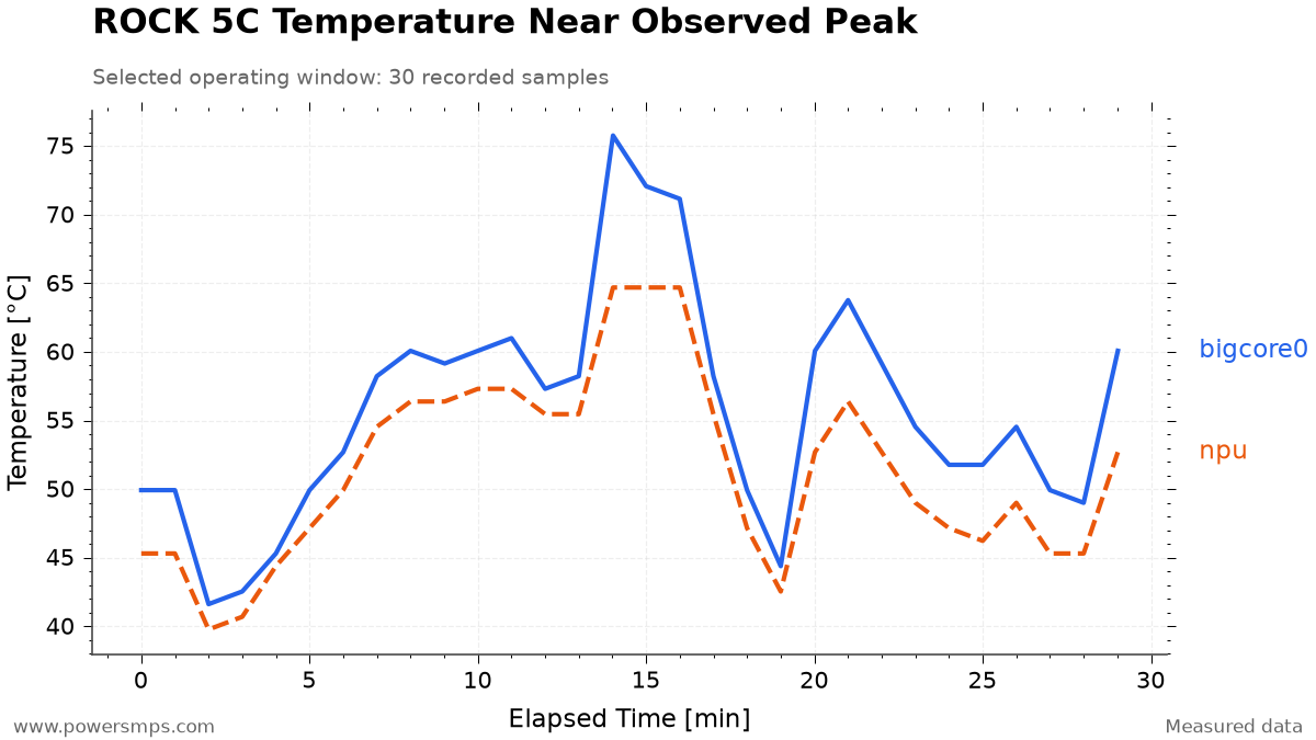
    Thermal shifts are more intuitive when visualized on a graph. Below are 30 samples selected from a 15-minute window around the point when bigcore0 reached its peak of 75.769°C.

    30 samples around the peak CPU sensor temperature on ROCK 5C: CPU in solid blue, NPU in dashed orange
    30 samples around the CPU sensor peak during ROCK 5C operation. Solid blue line represents CPU bigcore0; dashed orange line represents NPU temperature.

    The bigcore0 temperature hovered around 50°C, surged to a peak of 75.769°C at minute 14, and exhibited dynamic characteristics by dropping to 49.923°C at minute 18. Over the same interval, the NPU temperature sustained a peak of 64.692°C between minutes 14 and 16 before cooling down gradually.

    What stands out to me is how temperatures fluctuate dynamically with workload phases rather than staying at a static level. I am curious to see how this curve will differ on the RK3688. Alongside shorter waiting times, I also want to verify firsthand what degree of heatsink or fan cooling will be required for comfortable operation.

    Differences Between Single MatMul and Full Inference Performance

    On the Radxa ROCK 5C (RK3588 runtime target, RKNPU driver 0.9.8, RKNN Runtime 2.3.2), single-core benchmarks using the RKNN MatMul C API on primary shapes of the Anima DiT FFN block (Linear 1: M=1024, K=2048, N=8192 / Linear 2: M=1024, K=8192, N=2048, 34.36 GOP each) yielded the following results:

    Compute Path & Precision Linear 1 Latency Linear 2 Latency Combined Sum Speedup vs. FP16
    FP16 x FP16 -> FP16 51.89 ms 460.61 ms 512.50 ms 1.00x
    INT8 x INT8 -> INT8 19.13 ms 115.67 ms 134.80 ms 3.80x
    FP16 x FP16 -> FP32 57.93 ms 463.10 ms 521.03 ms 1.00x
    INT8 x INT8 -> INT32 100.80 ms 118.32 ms 219.12 ms 2.38x

    What caught my eye in this table is the second Linear layer. Although both operations comprise 34.36 GOP each, executing the dimension-reducing Linear 2 in FP16 took 460.61 ms. The sum for the INT8 I/O path was roughly 3.80× faster than FP16, and roughly 2.38× faster in the INT32 output comparison. It was intriguing to see that perceived performance can vary substantially depending on operator shape and precision, even on the very same board.

    In those tests, context creation was rejected for the W8A16 formats RKNN_FLOAT16_MM_INT8_TO_FLOAT32 and RKNN_FLOAT16_MM_INT8_TO_FLOAT16. When requesting core_mask=7 via the MatMul API, execution fell back automatically to a single core, and INT8 execution emitted a ‘failed to update out cvt offset!’ warning. Because of these experiences, I plan to verify supported precisions and actual core configurations first on the new board.

    What concerned me even more than speed was output quality. In the W8A8 Quality Degradation and 8GB Resident Context Experiment, images generated using FFN Linear W8A8 were visually unsatisfactory, forcing a return to the FP16 configuration. I also experienced toolchain-dependent discrepancies in the Comparison Between RKNN Toolkit 2.3.2 and 2.3.0. Therefore, on the RK3688, what I am most eager to see is not just the raw TOPS figure, but how much speed can be gained while fully preserving the visual fidelity of the current model.

    Five Tests to Repeat After Purchasing the RK3688

    Once I purchase the equipment, I plan to run the following five tests sequentially across both boards. Evaluating them under identical conditions alongside board-specific optimizations should clarify which configuration provides the best practical usability.

    The model, input prompt, precision, resolution, step count, and seed will be locked first. Documenting board revisions, memory specs, SDK versions, and cooling environments alongside them will make it straightforward to review the results later.

    Workload to RunWhat I Want to Observe
    Idle StateTemperatures and clocks under no load; standby power once metering equipment is prepared
    All-Core CPU LoadThroughput comparisons across identical thread counts vs. all available cores on each board, logging sustained clock speeds and temperatures
    Single NPU OperatorExecution latency and output numerical deviations across identical shapes and precisions; verifying actually accepted core configurations
    Full Anima InferenceEnd-to-end latency including model loading, encoding, denoising, and VAE; comparing cold vs. warm runs
    Long-Term Repeated OperationCounts of completions vs. failures, p50 / p95 latencies, alongside memory, swap, temperature, and clock variations

    Once a power meter is ready, I also want to log power consumption over time during generation to calculate the energy consumed per image. Executable hashes will be recorded per board, and original models and inputs will be strictly matched for comparison.

    Board-tailored optimizations, such as the Spectrum Optimization Technique, will be documented separately. This will allow assessing both baseline disparities and the most practical configurations for daily use.

    What I Expect from the RK3688

    How Many Minutes Will a 25.20-Minute Workload Take on the New Board?

    Separate from the mixed-setting averages, I revisited a Spectrum 20-step run where stage-by-stage timings had been logged. Under conditions of 512×512 resolution, CFG 4.0, and seed 20260812, applying Spectrum to FP16 DiT followed by CPU VAE decoding took 1356.58 s for denoising and 155.46 s for VAE. The two stages combined totaled 1512.04 s, or approximately 25.20 minutes. The time ranges below cover these two stages, excluding prompt encoding and model loading.

    I am hoping that this 25.20-minute baseline can be reduced to approximately 7~13 minutes on the RK3688. My primary projection centers around 9 minutes. Calculating with different acceleration assumptions for the denoising stage and CPU VAE yields the following:

    ScenarioDenoising Stage AssumptionCPU VAE AssumptionCombined Two-Stage Total
    Current ROCK 5C Measurement1356.58 s155.46 s25.20 min
    Conservative Expectation2× faster1.5× faster13.03 min projected
    My Median Expectation3× faster2× faster8.83 min projected
    Optimistic Case4× faster2.5× faster6.69 min projected

    The formula is 1356.58 s / denoising speedup multiple + 155.46 s / VAE speedup multiple. For instance, if overall denoising speeds up by 3× and CPU VAE speeds up by 2×, the total becomes roughly 8.83 minutes. These multiples represent scenarios I outlined based on the upgraded CPU, NPU, and memory specifications. In particular, proper support for FP16 operations and smooth integration with the RKNN toolchain will be necessary to approach the optimistic scenario.

    After acquiring the board, I plan to remeasure denoising and VAE timings under the same 20-step configuration and place them alongside this projection table. Dropping to around 9 minutes per image would substantially transform the interactive flow of revising prompts and generating images. If thermal performance and fan noise improve as well, satisfaction with the upgrade will be even higher.

    I look forward to seeing how significantly the RK3688 will alleviate long image generation latencies and memory pressure. If overall thermals, acoustics, and the ease of repeated execution improve alongside peak performance, the case for upgrading will become all the more compelling.

    Once purchased, I plan to systematically update this article with processing times, image quality, memory usage, and thermal results. After verifying whether these expectations hold true in practice, detailed configurations and troubleshooting steps will be continued in follow-up posts.

  • Smoothing Capacitor Lifetime Calculation: High-Temp PCBA Temperature Measurement, Layout, and Vent Clearance

    Smoothing Capacitor Lifetime Calculation: High-Temp PCBA Temperature Measurement, Layout, and Vent Clearance

    Smoothing capacitor lifetime cannot be evaluated solely from datasheet hour ratings. When evaluating a PCBA operating at high temperatures, the crucial criteria to verify firsthand are whether the temperature was measured under actual high-temperature conditions, and which input in the manufacturer’s lifetime formula that temperature corresponds to. Values obtained with an open board at room temperature must never be applied directly to the high-temperature operating conditions of the finished product.

    Temperatures must be measured directly using thermocouples, while also analyzing the heat flow from bridge diodes, SMPS power semiconductor devices, transformers, and heatsinks. Separately from lifetime calculations, the potential for short circuits with adjacent components or the chassis upon pressure vent actuation must also be evaluated. Based on this design experience, this article outlines the lifetime evaluation procedure for non-solid aluminum electrolytic smoothing capacitors using liquid electrolyte.

    Smoothing Capacitor Lifetime Calculations Begin by Verifying Datasheet Test Conditions

    In aluminum electrolytic capacitors, electrolyte gradually dissipates through the end seal during operation, which can cause capacitance to decrease and dielectric losses to increase. In typical smoothing circuits, ambient temperature and self-heating due to ripple current are the critical factors in lifetime evaluation. You must first verify the endurance test conditions of the selected series—including temperature, applied voltage, ripple current superposition, and end-of-life criteria. Nippon Chemi-Con Lifetime Technical Document

    A practical approximation formula describing the effect of temperature is given below. However, this equation alone does not calculate the final product lifetime reflecting all ripple current conditions.

    \[L_x=L_o\times B_t^{(T_o-T_x)/10}\]

    Here, \(L_o\) is the specified lifetime under datasheet test conditions, and \(L_x\) is the estimated lifetime under operating conditions. \(T_o\) is the upper category temperature, \(T_x\) is the actual ambient temperature defined in the manufacturer’s model, and \(B_t\) is the temperature acceleration factor. Corrections for ripple self-heating and applicable limits must be verified using product-specific lifetime formulas or calculation tools.

    The commonly cited rule of thumb that ‘when temperature drops by 10°C, lifetime approximately doubles (2x)’ is an approximation assuming \(B_t=2\). Nippon Chemi-Con explains this approximation over an ambient temperature range of roughly 60~95°C, noting that products with maximum operating temperatures of 105°C or higher may require coefficient corrections depending on the estimated temperature range. You should never apply the same coefficient across all series and temperature ranges, nor should calculation results be interpreted as guaranteed lifetime.

    For basic selection of capacitance, rated voltage, and permissible ripple current, it is helpful to cross-reference our previous article, How to Select Smoothing Capacitors.

    Three Temperatures to Measure on a High-Temperature PCBA

    For PCBAs operating at elevated temperatures, the fundamental principle is to take measurements under replicated operating conditions. Maintain the actual chassis, enclosure covers, mounting orientation, and cooling conditions, and record expected input, output, and load conditions. For continuous-duty products, evaluate conditions only after temperatures have fully stabilized. Do not assume that maximum load alone represents the most severe thermal condition for all components; define test conditions tailored to the product’s actual operating envelope.

    Before plugging values into a lifetime equation, you must distinguish between the following three temperatures. The ambient temperature description below is based on Nippon Chemi-Con’s measurement definitions; always verify the definitions provided by the specific manufacturer selected for your application.

    Category Definition Key Considerations in Lifetime Evaluation
    Ambient Temperature The temperature at the specific mounting location influenced by external convection, radiation, and conduction, excluding self-heating of the capacitor Cannot be assumed to be equal to room ambient air temperature
    Case Surface Temperature Temperature measured on the capacitor outer can during operation Reflects both ambient thermal effects and internal self-heating, so it must not be directly substituted as ambient temperature
    Core Temperature Temperature of the internal capacitor element Must not be assumed identical to surface temperature; evaluate according to manufacturer-approved methodologies

    Power loss due to ripple current can be approximated as follows. Because the resulting internal temperature rise directly impacts lifetime, one must not conclude the design is safe based solely on a low ambient temperature.

    \[P\approx I_{\mathrm{rms}}^2\times\mathrm{ESR}\]

    Entering the operating surface temperature into the ambient temperature field while adding ripple self-heating again can result in double-counting thermal rise. Conversely, one should never omit evaluating internal temperature simply because surface temperature appears acceptable. The first step is to record whether each measured value corresponds to ambient, surface, or core temperature, and align it with the input definitions of the manufacturer’s lifetime model.

    Contact and Operating Condition Replication Are Critical When Measuring with Thermocouples

    Directly measuring temperatures used for lifetime evaluation with thermocouples is critical. However, using a thermocouple does not automatically guarantee accurate measurements. You must verify sensor contact and mechanical fastening, instrument calibration status, and electrical insulation. Documenting the attachment location alongside test conditions ensures that thermal performance before and after layout modifications can be compared on the same baseline.

    Nippon Chemi-Con introduces a methodology that uses thermal imaging to identify locations under high thermal stress, followed by dummy capacitors and multiple thermocouples to evaluate external thermal influences excluding self-heating. The key principle is never to label operating can surface values directly as ambient temperature. For detailed specialized measurement procedures, follow the manufacturer’s guide to ambient temperature measurement.

    Opening chassis covers or altering fan and ducting configurations to route thermocouple leads alters the actual thermal environment. Even after attaching sensors, you must recreate the final assembled enclosure and cooling conditions, verifying that temperatures reach steady state. Sensor attachment points should conform to manufacturer guidelines, and stabilization soak time must be determined based on when the system reaches true thermal equilibrium.

    Sensor attachment and repositioning must be performed only after disconnecting power and verifying that residual voltages are fully discharged. When measuring power supply sections, verify insulation integrity across the sensors, instrumentation, and cabling. Never attempt to measure internal temperatures by modifying capacitor construction or probing charged terminals directly.

    Component Placement Considering Convection from Bridge Diodes and Heatsinks

    Smoothing capacitors are typically surrounded by heat-generating components such as bridge diodes, SMPS power semiconductors, and transformers (TRANS). Experience shows that checking physical clearance between components is not enough. You must also trace the pathways through which heat escaping from heat-generating components and their heatsinks reaches the capacitor.

    Thermal flow paths differ significantly between natural convection and forced-air cooling, and product mounting orientation exerts a major influence. Verify that the capacitor does not lie in the exhaust path of hot air discharged from heatsinks based on the actual installed orientation. After modifying the component layout, remeasure under identical operating conditions to verify that thermal stress has been reduced.

    In addition to convection, radiative heat transfer and thermal conduction through the PCB must be considered. Nichicon advises against placing heat-dissipating components near electrolytic capacitors or directly beneath capacitors on the reverse side of the board. The more constrained the layout area, the more critical it is to jointly examine surrounding heat sources and cooling airflow paths. Nichicon Application Guidelines

    Vent Clearance: Operating Margin and Secondary (2nd) Short-Circuit Prevention Are Evaluated Separately

    Failure conditions where internal pressure rises due to electrolyte vaporization or gas generation must be taken into account. The pressure vent is a safety mechanism designed to mitigate the risk of violent case rupture caused by excessive internal pressure buildup. In engineering practice, designers must evaluate whether deformed can sections will contact adjacent components or the chassis upon vent opening, and whether venting electrolyte can bridge conductors and cause electrical short circuits.

    Examples of minimum top clearance above the vent recommended by Nippon Chemi-Con are outlined below. Individual product specifications and exceptions must be consulted first. These dimensions represent mechanical clearance to avoid impeding vent operation; they do not guarantee electrical insulation or safety against electrolyte expulsion. Pressure Vent and Top Space Guidelines

    Case Outer Diameter Example Minimum Top Clearance Above Vent
    8 mm (some 6.3 mm products) to 16 mm 2 mm or more
    18~35 mm 3 mm or more
    40 mm or more 5 mm or more

    Nichicon instructs that circuit traces and wiring must not be routed over the vent, explaining that because electrolyte is conductive, contact with the PCB creates risks of smoke and fire due to trace corrosion or short circuits. Therefore, design reviews must not stop at verifying overhead clearance dimensions; the actual vent orientation and expected spray paths must also be investigated.

    In the final layout, designers must jointly evaluate vent opening orientation, expansion deformation envelope, component and chassis locations with assembly tolerances, potential electrolyte dispersion paths, operating voltages, and finished-product safety requirements. Electrical clearance and creepage distances are entirely separate considerations from vent mechanical clearance. Because no single safety spacing rule applies universally across all mechanical enclosures, the final clearance must be determined based on component manufacturer data and the specific product architecture.

    A clear distinction must also be made between end-of-life dry-up and vent actuation caused by abnormal pressure buildup. Gradual wear-out degradation, where electrolyte loss leads to decreased capacitance and increased loss tangent, does not necessarily culminate in vent opening. Lifetime calculations evaluate parametric degradation, whereas layout reviews serve to mitigate secondary (2nd) damage during fault events such as vent actuation.

    Comparison of Relative Lifetime Ratios with Decreasing Temperature

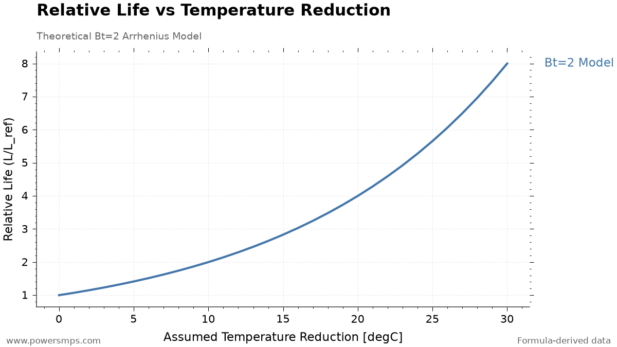
    The following is an educational calculation assuming \(B_t=2\) with all other conditions held constant. It does not represent actual measurement data or guaranteed lifetimes for a specific product. Relative lifetime ratios were calculated based on temperature reduction relative to a baseline. The applicable temperature range and ripple corrections must be verified for each specific product series.

    \[\frac{L}{L_{\mathrm{ref}}}=2^{\Delta T_{\mathrm{red}}/10}\]
    Assumed Temperature Reduction Calculated Relative Lifetime Ratio
    0°C 1x
    10°C 2x
    20°C 4x
    30°C 8x
    Relative lifetime ratio versus temperature reduction assuming Bt=2. Educational calculation; not an actual measurement or guaranteed lifetime for a specific product.
    Relative lifetime ratio versus temperature reduction assuming Bt=2. Educational calculation; not an actual measurement or guaranteed lifetime for a specific product.

    This comparison illustrates why engineers verify operating temperatures with thermocouples and scrutinize the placement of heat sources. In practical design, one must not apply these multiplier ratios directly to product lifetime simply because the temperature was reduced; always re-evaluate using the specific lifetime model for the chosen series.

    When completing the design review, verify the following checklist items.

    • Have high-temperature operating conditions, the actual chassis enclosure, mounting orientation, and cooling airflow been faithfully replicated?
    • Have thermocouple mechanical contact, secure fastening, instrument calibration status, and electrical insulation been verified?
    • Have ambient, case surface, and core temperatures been clearly distinguished, ensuring self-heating is not double-counted?
    • Have the manufacturer’s series endurance test conditions and lifetime equation validity boundaries been confirmed?
    • Has thermal airflow from bridge diodes, transformers, SMPS power semiconductors, and heatsinks been fully considered?
    • Have vent operational clearance and clearance to prevent short circuits to adjacent components and the chassis been evaluated separately?
  • Hindsight Operating Costs: Why We Chose APIs for Embeddings and Local NPU for Reranking

    Hindsight Operating Costs: Why We Chose APIs for Embeddings and Local NPU for Reranking

    While operating Hindsight in Docker, we use cloud APIs for the LLM and embeddings, and run the reranker on a local NPU. Because embedding API costs are low, we saw no need for local operation, whereas the reranker was moved locally to avoid recurring API expenses.

    While running Hindsight, a Docker-based long-term memory management system, on a single-board computer (ROCK 5C, RK3588 SoC, 8GB RAM), we adopted a hybrid architecture that splits cloud APIs and the local NPU according to workload characteristics. LLM generation and embeddings are handled via commercial APIs, while candidate reranking during retrieval is processed on the local NPU.

    Across 9 complete UTC calendar days, the gateway recorded 12,536 requests of production traffic; based on these logs and hardware benchmark data, this article outlines the economic and technical rationale and latency trade-offs behind this partitioned design.


    1. Hybrid Architecture: Partitioning LLM and Embedding APIs from the Local NPU Reranker

    The criteria for distributing each inference task in the Hindsight environment stems from the interaction between hardware resource requirements and API pricing models.

    • Generative LLM: We use the DeepSeek V4.1 Flash cloud API via OpenCode Go. Within the monthly subscription usage limits, usage is metered at peak rates (input $0.30 per 100 ten-thousand tokens, output $1.20, cache read $0.006) and off-peak rates (with a 50% discount applied).
    • Text Embeddings: We use the Google Gemini Embedding 2 (768-dimensional) cloud API.
    • Document Reranker: By leveraging the local NPU of the single-board hardware (Rockchip RK3588, RKLLM 1.2.1), we run Qwen3-Reranker-0.6B.

    Model execution and memory constraints on the same board were also examined in Limitations of Anima RKNN Optimization: W8A8 Quality Failure and 8GB Resident Model Experiment and Generating Anima Images on RK3588: RKNN Conversion and Execution Results on ROCK 5C 8GB.

    Communication between Hindsight and upstream models is proxied through Bifrost (v2.2.4), a central LLM gateway. For the reranker, to avoid the compounding unit cost of continuously calling commercial cloud APIs, we used the Qwen3-Reranker-0.6B model released by Alibaba Cloud’s Qwen team, converted into the RK3588-dedicated W8A8 quantized format (.rkllm) distributed by the community (Hugging Face dulimov). We wrapped and connected this model as a Cohere-compatible HTTP service based on a native C++ logit bridge (RKLLM_INFER_GET_LOGITS) in an isolated Docker Compose container.


    2. Bifrost Logs: Requests and Cost Scope Across 9 Days

    In Bifrost’s Hindsight-dedicated virtual key logs from 2026-10-14 00:00:00Z through 2026-10-23 00:00:00Z across 9 UTC dates, we examined requests. The table below summarizes only the successful requests for Gemini Embedding 2 and the active DeepSeek V4.1 Flash within this window.

    Provider and Model Successful Requests Prompt Tokens Completion Tokens Total Tokens Bifrost Recorded Cost (USD)
    gemini / gemini-embedding-2 9,484 1,307,222 0 1,307,222 $0.2614
    opencode-go / deepseek-v4.1-flash 889 6,833,856 2,754,646 9,588,502 $2.5412

    Both amounts represent recorded figures calculated from unit rates configured in the gateway. For Gemini as well, actual billing may vary depending on the account’s free tier quotas and other terms.

    First, for DeepSeek V4.1 Flash under OpenCode Go, the metered amount ($2.5412) is an equivalent value calculated by the gateway to manage token usage quotas according to the provider’s time-of-day tariff schedule (peak and 50% off-peak discount). It does not reflect the operator’s actual monthly subscription invoice amount.

    Second, for Gemini embeddings, we used logs after backfilling token and cost tracking. Previously missing records were not treated as free usage.

    Third, across the same observation window, the local Qwen reranker handled 731 successful requests. This configuration does not make external pay-as-you-go API calls for reranking. We did not interpret the absence of reranker token aggregation as meaning that token usage was 0.

    The total of 12,536 requests includes initial environment setup, load testing, retries, background jobs, and legacy proxy paths. We did not aggregate routes lacking cost records into an overall operating expense, nor did we extrapolate this table into daily/monthly averages or per-unit costs for storing or recalling a single memory.


    3. Why We Kept Embeddings on Cloud APIs: 130 Ten-Thousand Tokens for $0.26

    According to Google’s official pricing policy, the standard paid tier for Gemini Embedding 2 text is $0.20 per 100 ten-thousand input tokens (the asynchronous Batch API is $0.10, but Hindsight’s synchronous pipeline is billed at standard rates).

    Over 9 UTC days, Gemini prompt tokens consumed by Hindsight for memory storage and query processing totaled 1,307,222. Calculating this using the official standard unit rate yields the following:

    \[1,307,222 \times \frac{\$0.20}{1,000,000} = \$0.2614444\]

    The value calculated at standard unit rates is $0.2614444. The $0.2614 in the table reflects this rounded. Within this observation window, the recorded expense corresponding to 9,484 successful embedding requests was approximately $0.26.

    At this usage volume, embedding API costs remain low enough that we saw no need to operate an additional local model. We decided to keep embeddings on the API while focusing local resources and operational maintenance on the reranker. This decision reflects our current setup and traffic volume.


    4. Why We Moved the Reranker Locally: Qwen3 RKLLM NPU Performance and Measured Latency

    The initial motivation for migrating the reranker locally was API cost pressure. Under our current operating environment, we remain satisfied with Qwen’s retrieval result quality and continue to use it. This was not calculated as cost savings directly compared against the pricing of any specific commercial reranker.

    The local reranker environment runs on the ROCK 5C single-board computer using its RK3588 NPU and RKLLM 1.2.1 runtime. We loaded the community-distributed dulimov/Qwen3-Reranker-0.6B-rk3588-1.2.1 W8A8 quantized model, invoking RKLLM_INFER_GET_LOGITS from a native C++ bridge to apply softmax over the tokenizer’s yes/no logits for score generation. We capped the context length to 2048 tokens, adding a guardrail that returns a 422 error when exceeded.

    In those benchmarks, runtime initialization took 2.283 seconds excluding Python module imports, and peak process RSS reached 1,437,372 KiB (approximately 1.371 GiB). This value represents the RSS of that process and differs from whole-system memory utilization.

    To validate quality, across 12 handcrafted test cases consisting of Korean and cross-lingual question-document pairs, we compared ranking accuracy against the existing CPU-based MiniLM (batch size 32). Out of 12 queries, for 11 queries the Qwen3 NPU model ranked the ground-truth document at rank 1 (ground-truth rank 1 ratio 11/12, MRR 0.9375), exhibiting higher discriminatory performance compared to MiniLM’s ground-truth rank 1 in 6 queries (ground-truth rank 1 ratio 6/12, MRR 0.6417) (note that these 12 test cases serve as pipeline integration validation probes and do not guarantee public IR benchmark scores).

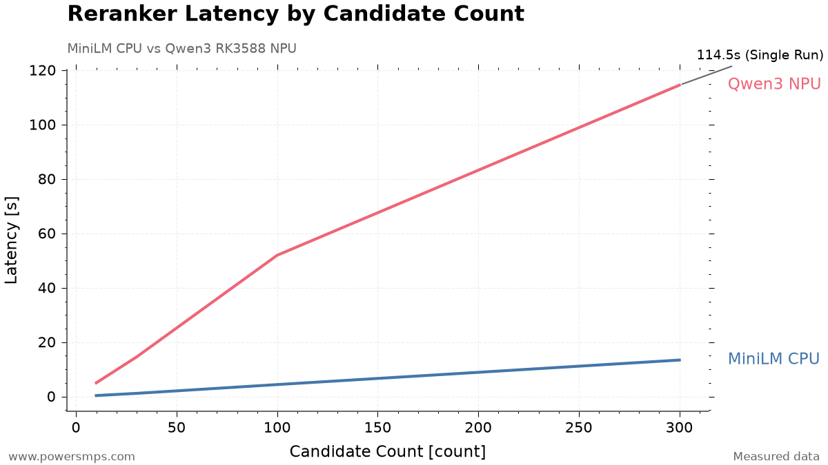
    In contrast, inference latency revealed clear limitations stemming from the serialized compute pipeline of the NPU model.

    Candidate Documents MiniLM CPU (Batch Size 32) Qwen3 RK3588 NPU (Single Serial Inference)
    10 0.372 s (median of 3 runs) 5.047 s (median of 3 runs)
    30 1.175 s (median of 3 runs) 14.544 s (median of 3 runs)
    100 4.411 s (1-run observation) 51.980 s (1-run observation)
    300 13.423 s (1-run observation) 114.537 s (1-run observation)
    Comparison of execution latency across candidate counts between MiniLM CPU (batch size 32) and Qwen3-Reranker-0.6B RK3588 NPU (serial execution). Data for 10 and 30 candidates represent medians of three runs; 100 and 300 candidates are single shared-host observations.
    Comparison of execution latency across candidate counts between MiniLM CPU (batch size 32) and Qwen3-Reranker-0.6B RK3588 NPU (serial execution). Data for 10 and 30 candidates represent medians of three runs; 100 and 300 candidates are single shared-host observations.

    Tests across candidate counts were constructed by repeating 48 short documents on a shared host. Total prompt input for Qwen averaged approximately 108 tokens. Each implementation used its own prompt structure and tokenizer, with MiniLM executing at batch size 32 while Qwen processed candidates serially. The results in the table reflect empirical observations from benchmarking these two implementations.


    5. Real-World Operational Strategy: Retaining the Local Reranker Despite Slow NPU Inference

    For processing 100 candidates, a latency of 52 seconds represents significant wait time from the standpoint of real-time conversational services. Nevertheless, the decision to retain this setup in production rests on the operator’s specific workflow characteristics and concrete optimization configurations.

    In actual everyday use, the perceived slowdown is negligible, so we continue using Qwen due to its satisfactory quality. This assessment reflects our specific operating workflow; it cannot be generalized to suggest that the latency figures measured above are universally short.

    To preserve system stability, we enforced two core operational policies.

    1) Upfront Candidate Capping at 50 Documents

    In the initial configuration, up to 300 candidate documents were forwarded to the reranker. In a real-world memory recall benchmark where 244 candidates were passed, reranking alone consumed 181.868 seconds, driving total recall latency to 183.612 seconds.

    We subsequently applied HINDSIGHT_API_RERANKER_MAX_CANDIDATES=50 in Hindsight’s configuration to restrict the Reciprocal Rank Fusion (RRF) stage so that only the top 50 candidates are passed to the reranker. Re-testing with the identical query reduced reranking latency to 104.259 seconds (a 42.67% reduction) and total memory recall latency to 105.791 seconds (a 42.38% reduction). Because these figures originate from distinct inputs and measurement conditions, they cannot be directly compared against the preceding short-document benchmark latencies.

    Single-Execution Comparison on Identical Query Previous Configuration (Max 300 Allowed, 244 Evaluated) Capped Configuration (50 Upfront Cap, 50 Evaluated)
    Evaluated Candidate Documents 244 50
    Reranking Execution Time 181.868 s 104.259 s
    Total Memory Recall Time 183.612 s 105.791 s
    Final Returned Memories 48 44
    Original Source Memory Rank Rank 1 Rank 1

    Although the candidate count decreased from 244 to 50, reduced to roughly a 5-to-1 ratio, execution time did not scale down proportionally. This disparity is likely driven by compound factors such as prompt cache reuse rates and background resource contention on the shared single-board host; linear latency scaling with respect to candidate counts should not be assumed as a performance guarantee. Capping the candidate pool at 50 carries the trade-off of potentially excluding relevant memories from reranking in exchange for lower latency.

    2) Gateway Serial Queueing and Multi-Tier Timeouts

    To ensure that the local worker processes only one request at a time, we configured Bifrost’s reranker concurrency to 1 and channel buffer to 10. Under current global policy, additional requests can still wait when the buffer fills, meaning buffer 10 does not represent an absolute upper bound on total queued requests.

    In actual synthetic load testing (sequential arrival of 16-document requests (1 call) and 2-document requests (10 calls)), all 11 requests succeeded within the 33.2~35.1-second range with HTTP 200, and the NPU worker process was stably reused without restarts.

    We also established multi-tier timeout margins to prevent unexpected NPU lockups.

    • Hindsight reranker timeout: 1800 s (30 min)
    • Bifrost upstream socket timeout: 780 s
    • Local native C++ inference timeout: 600 s
    • Native queue wait timeout: 120 s

    These timeout values do not represent nominal system response latency, but rather safety margins configured to recover and restart processes safely when requests stall in queues or encounter abnormal delays.


    6. Operational Limits and Decision Criteria: Workload Partitioning in Single-Board LLM Systems

    Whether to retain a local reranker must be judged by jointly evaluating API expenditure, retrieval quality, and latency overhead. The rationale and operational limitations of maintaining the current architecture are summarized below.

    We also benchmarked KURE’s fixed 256-token FP16 RKNN model. Across the identical 50 inputs, HTTP rerank response latency was 10.647 s for KURE and 27.798 s for Qwen. However, KURE truncated documents across 2 inputs, and subsequent live recall tests yielded different final rankings. These samples do not conclusively prove overall quality superiority between the two models. For now, we continue using Qwen.

    Second, there are limitations to the benchmark sample. The ranking performance observed in this operational deployment—ground-truth rank-1 hit count of 11/12 (Top-1 hit rate) and MRR 0.9375 ranking performance—reflects only minimum pipeline verification probe results for service deployment, and does not represent generalized retrieval efficacy on large-scale Korean information retrieval (IR) datasets.

    Our decision criteria in this operational setup are as follows:

    1. Embeddings: At current usage levels, API costs remain low enough that we saw no practical necessity for local operation.
    2. Reranker: We chose local Qwen due to API cost burdens. We continue to run it because we are satisfied with its quality and perceive no noticeable slowdown in real-world use.

    Under our present workload, there is ample justification to keep embeddings on cloud APIs, while cost and quality warrant keeping the reranker local. Should traffic volume or response-latency constraints change, this architectural division can be re-evaluated.

  • Anima RKNN Inference Optimization: Reducing Generation Time by 41% with Spectrum

    Anima RKNN Inference Optimization: Reducing Generation Time by 41% with Spectrum

    Affiliate Disclosure: This post contains AliExpress affiliate links. If you make a purchase through these links, the author may receive a commission.

    1. Reducing Image Generation Time

    When running large-scale Diffusion Transformers (DiT) on-device in a single-board computer (SBC) environment, memory constraints and computation time are the primary bottlenecks. Using a Radxa ROCK 5C 8GB board purchased directly from the official Radxa AliExpress store, we conducted Anima DiT inference optimization experiments based on the 2026-8 environment.

    Denoising a 512×512 image for 20 steps took 2,408.54 seconds. Including the time required to reconstruct the image with the VAE, generating a single image exceeded 30 minutes. A method was needed to reduce the computational workload while preserving the visual quality of the output.

    We applied Spectrum to the FP16 RKNN configuration executed in Part 1. While retaining the Euler scheduler, we replaced model computations on selected steps with predictions based on prior results, and compared the speed and image quality.

    2. Hardware and Model Configuration Used for Comparison

    The experimental hardware is the Radxa ROCK 5C single-board computer, equipped with a Rockchip RK3588S2 SoC and 8GB of system memory.

    The RKNN runtime target is rk3588. The test device is the ROCK 5C 8GB, which must be distinguished from the ROCK 5C Lite listed on the same product page.

    We used 84 FP16 RKNN models, partitioning Anima’s 28 DiT blocks into self-attention, cross-attention, and FFN subgraphs. The underlying conversion structure is identical to the setup described in Part 1.

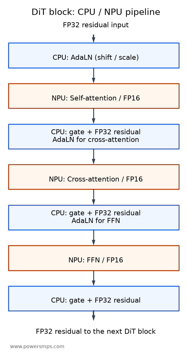
    The NPU processes primary matrix and attention operations. The CPU handles AdaLN, FP32 residual accumulation, the Euler scheduler, text encoding, and VAE decoding. This division of roles was maintained even after adding Spectrum.

    3. What Computations Does Spectrum Skip?

    Spectrum is not a sampler that replaces Euler. It is a caching technique that predicts the denoised state of the current step from prior computational results to reduce model recalculations. We ported the Spectrum implementation from stable-diffusion.cpp to NumPy and integrated it into the Euler loop.

    The core principle of Spectrum leverages the property that latent variable trajectories do not change abruptly between steps during diffusion, forecasting an estimate of the denoised state \(x_0\) from a prior history buffer.

    At each step, the pipeline selects between direct computation and prediction. Both paths feed their results into the same Euler scheduler.

    • On directly computed steps, conditional and unconditional outputs are combined via CFG, and the denoised state is calculated as x₀ = xₜ − σ × prediction and stored in the history buffer.
    • On prediction steps, the current x₀ is estimated from prior history, skipping NPU model computation entirely.
    • The estimated x₀ is converted back into a flow prediction via prediction = (xₜ − x₀) / σ. Both paths update the next state using the same Euler integrator.

    Thanks to this architecture, the scheduler itself retains the FlowMatch Euler formulation while substantially reducing the number of tensor operations dispatched to the NPU.

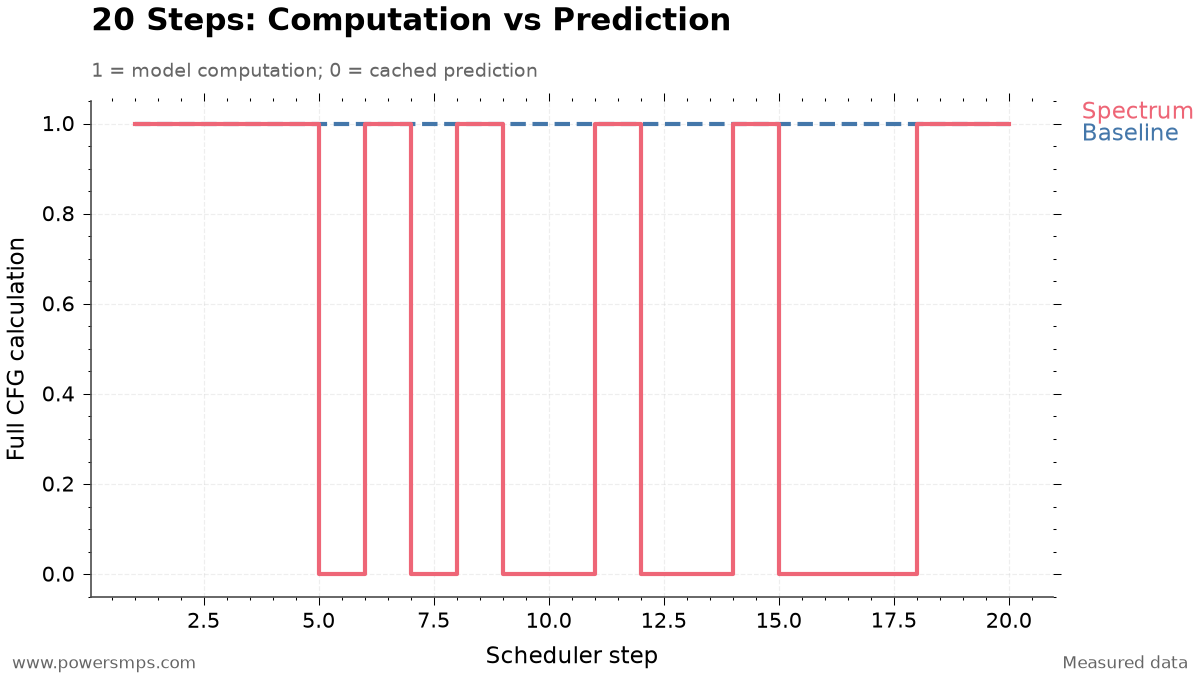
    4. 20 Steps: 11 Computations, 9 Predictions

    Across a 20-step run, the steps computed directly and those replaced with predictions are broken down as follows:

    • Actual model computation steps (11 steps): Step 1, 2, 3, 4, 6, 8, 11, 14, 18, 19, 20
    • State prediction skipped steps (9 steps): Step 5, 7, 9, 10, 12, 13, 15, 16, 17

    The first 4 steps were all directly computed to accumulate the history required for forecasting. In the intermediate phase, 9 steps were replaced with predictions, and the final 18~20 step was directly computed again.

    20-Step Sampling Policy: Baseline vs Spectrum Forecasting
    20-Step Sampling Policy: Baseline vs Spectrum Forecasting

    Here, 11 computation steps do not translate to just 11 NPU executions. Each CFG step requires separate DiT evaluations for conditional and unconditional inputs.

    Because each transformer evaluation traverses 84 RKNN subgraphs across 28 blocks, 1 CFG evaluation requires 168 subgraph NPU executions (84 × 2). Therefore, the 11 model computations in the Spectrum pipeline represent the following actual hardware traversal volume:

    • Full model passes (Transformer Passes): 11 passes × 2 = 22 passes
    • Subgraph NPU execution count: 11 passes × 2 × 84 subgraphs = 1,848 executions

    By contrast, the baseline pipeline executes 40 transformer passes and 3,360 subgraph NPU executions across 20 steps. In other words, Spectrum eliminated exactly 18 model passes and 1,512 subgraph executions, significantly cutting hardware load.

    5. Benchmark Results: Total Generation Time Reduced by 41.02%

    The baseline and Spectrum were evaluated on the same ROCK 5C 8GB. The resolution (512×512), 20 steps, CFG scale of 4.0, and seed 20260812 were kept strictly identical.

    Metric Baseline Non-cached FP16 RKNN + sd-cpp VAE Spectrum Accelerated Pipeline Difference & Speedup
    20-Step Denoise Latency 2,408.54 seconds 1,356.58 seconds 1,051.96 seconds saved (43.68% reduction, 1.775× speedup)
    sd-cpp Tiled CPU VAE Decoding 155.04 seconds 155.46 seconds +0.42 seconds (comparable run-to-run variance)
    Total Elapsed Time (Excluding Prompt Encoding) 2,563.58 seconds 1,512.04 seconds 1,051.54 seconds saved (41.02% reduction, 1.695× speedup)

    The measured figures highlight the following bottleneck and optimization characteristics:

    1. Concentration of Denoising Acceleration: Net 20-step denoise latency decreased from the baseline of 2,408.54 seconds to 1,356.58 seconds with Spectrum, saving 1,051.96 seconds. This represents a 43.68% time reduction and a 1.775× speedup. This achieves near-linear acceleration efficiency, closely matching the proportion of skipped operations (45%, or 9 out of 20 steps).
    2. Independence of VAE Decoding: The lightweight tiled CPU VAE decoder from sd-cpp, powered by ARM NEON/OpenMP via the ggml backend, took 155.04 seconds for the baseline and 155.46 seconds for the Spectrum pipeline—a difference of just 0.42 seconds. In this benchmark, VAE decoding time remained essentially identical, confirming that the performance gains were concentrated almost exclusively in the denoising stage.
    3. Full-Pipeline Speedup: Excluding prompt encoding, total end-to-end pipeline latency dropped from the baseline of 2,563.58 seconds (approximately 42 minutes 43 seconds) to 1,512.04 seconds (approximately 25 minutes 12 seconds), saving 1,051.54 seconds. The complete generation pipeline achieved a 41.02% reduction and a 1.695× speedup, successfully fulfilling the project target of generating images in under 30 minutes.

    6. What Is the Image Quality of the Accelerated Output?

    Caching algorithms that perform step prediction carry the risk that accumulated error might cause the latent space to diverge or produce invalid numerical values (NaN, Inf). Therefore, immediately upon pipeline completion, we conducted staged verification covering both numerical integrity of the output tensors and image-level visual quality.

    Neither NaN nor Inf occurred in the final latent variables after completing all 20 steps. Numerical stability was confirmed independently of the final image’s visual fidelity.

    The generated 512×512 image met the visual quality criteria established for this experiment. Under these tested conditions, we therefore achieved acceptable output while significantly cutting generation time.

    This visual assessment is limited to a single validation run (1 run) under specific conditions (512×512 resolution, 20 steps, Guidance Scale 4.0, Seed 20260812). Spectrum’s \(x_0\) prediction is not mathematically lossless, and slight latent-space errors are introduced by the approximation. Consequently, these findings do not imply exact numerical identity with the baseline, nor do they guarantee lossless quality free from visual degradation across arbitrary prompts and seeds.

    7. Comparing with the Baseline Using Identical Weights

    Spectrum modifies which steps are directly evaluated; it does not requantize or convert model weights.

    Because it operates on the identical 84 FP16 RKNN models, disabling prediction caching immediately reverts execution to the full-step baseline.

    • Compare outputs with caching enabled versus disabled using the same prompt, seed, and step count.
    • Verify both numerical stability and the visual quality of the resulting image.
    • If output quality fails to meet expectations under new conditions, disable prediction and compute all steps.

    Under the tested conditions, total generation time decreased by 41.02%. When applying this technique to other prompts and seeds, results should always be compared against the baseline. In Part 3, we examine alternative optimizations that reduced execution time but were discarded due to visual quality degradation or memory overhead.

  • Limits of Anima RKNN Optimization: W8A8 Quality Failure and 8GB Resident Model Experiments

    Limits of Anima RKNN Optimization: W8A8 Quality Failure and 8GB Resident Model Experiments

    Affiliate Disclosure: This post contains AliExpress affiliate links. If you make a purchase through these links, the author may receive a commission.


    1. Two Attempts for Faster Inference

    After executing Anima inference on the ROCK 5C 8GB, we compared two optimizations: FFN quantization and resident model contexts. The board is equipped with an RK3588S2, and experiments were conducted in 2026-8 in the RKNN-Toolkit2 2.3.2 environment.

    We used the same 84-model FP16 RKNN partitioned configuration as in Part 1 as our baseline. The NPU processes attention and FFN, while the CPU handles AdaLN and FP32 residual accumulation. The questions addressed here are whether we can accelerate computation or reduce the repetitive model staging overhead.

    The architecture of sequentially executing 84 subgraphs at a fixed 512×512 resolution introduces inherent overhead from loading, initializing, and releasing models at every step. Accordingly, we established two core hypotheses for system optimization: 1. Compute Acceleration Hypothesis: Apply W8A8 integer quantization to the computationally heavy FFN layers to shorten NPU execution time. 2. Lifecycle Reduction Hypothesis: Keep the runtime contexts of all 84 RKNN models resident in memory (Resident Context) to eliminate repetitive loading and initialization time at each step.

    Empirically testing these two approaches on the ROCK 5C 8GB revealed concrete bottlenecks: image quality degradation and physical memory limits.


    2. Reducing Denoising Time by 18.48% with FFN Quantization

    We applied integer quantization to the FFN (Feed-Forward Network) regions of the 28 blocks where compute is concentrated, out of the total 84 RKNN subgraphs in the DiT. We adopted a hybrid build approach: weights and activations of the Linear(2048→8192) and Linear(8192→2048) layers inside the FFN were quantized to INT8 (W8A8), while the non-linear GELU activation and branch output sections were maintained in FP16. The self-attention and cross-attention cores retained their existing FP16 configuration, and the host-side residual stream also preserved FP32 precision.

    For quantization calibration, we used activation tensors collected during the baseline FP16 denoising process. Combining high/low sigma steps and conditional/unconditional CFG branches, we collected 4 sets per block for a total of 112 sets. All 28 FFN blocks were successfully converted.

    Under identical conditions—same initial latent (seed: 20260812), prompt context, CFG scale of 4.0, and 20 steps—the comparative benchmark results are as follows.

    Metric Baseline FP16 FFN Linear W8A8 Delta
    20-Step Denoise Time 2,408.54 seconds 1,963.45 seconds Reduced by 445.09 seconds (18.48% improvement)
    Average Time per Step 120.40 seconds 98.15 seconds Reduced by 22.25 seconds
    Average FFN Core Execution per Step 44.76 seconds 23.57 seconds 1.90× speedup
    Average Self Core Execution per Step 24.00 seconds 25.74 seconds Run-to-run variance level
    Average Cross Core Execution per Step 7.45 seconds 7.69 seconds Run-to-run variance level

    Overall denoising became 1.227× faster, and the quantized FFN section accelerated by 1.90×. No NaNs or Infs occurred during execution.


    3. Faster Execution, but Below Quality Standards

    Although denoising time decreased by 18.48%, the resulting 512×512 image after VAE decoding failed to meet visual quality criteria.

    Numerical stability without divergence was a separate matter from sufficient image quality. While this W8A8 configuration maintained numerical stability, it failed the image quality threshold.

    Therefore, we did not adopt FFN quantization and reverted to the FP16 configuration. Optimization of generative models must evaluate final image quality alongside execution latency.


    4. Time Reductions Possible by Keeping Models in Memory

    To reduce inference latency without degrading image quality, the next hypothesis evaluated was runtime model residency (Resident Context), which eliminates the loading and initialization overhead across the 84 subgraphs.

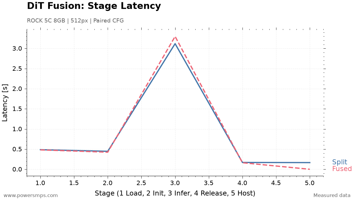
    The partitioned configuration loads each model, initializes the runtime, executes inference, and then releases it. The average preparation and teardown overhead across a single pass through all 84 models, measured over 3 runs, is as follows.

    Lifecycle Stage Elapsed Time for 1 Pass Across 84 Models (Average) Notes
    load_rknn 13.96 seconds Load model weights into host memory
    init_runtime 12.90 seconds Create NPU driver context and establish DMA mappings
    release 4.84 seconds Tear down NPU runtime and device mappings
    Pure Stage Sum 31.71 seconds Wall-clock time including loop overhead: 33.84 seconds

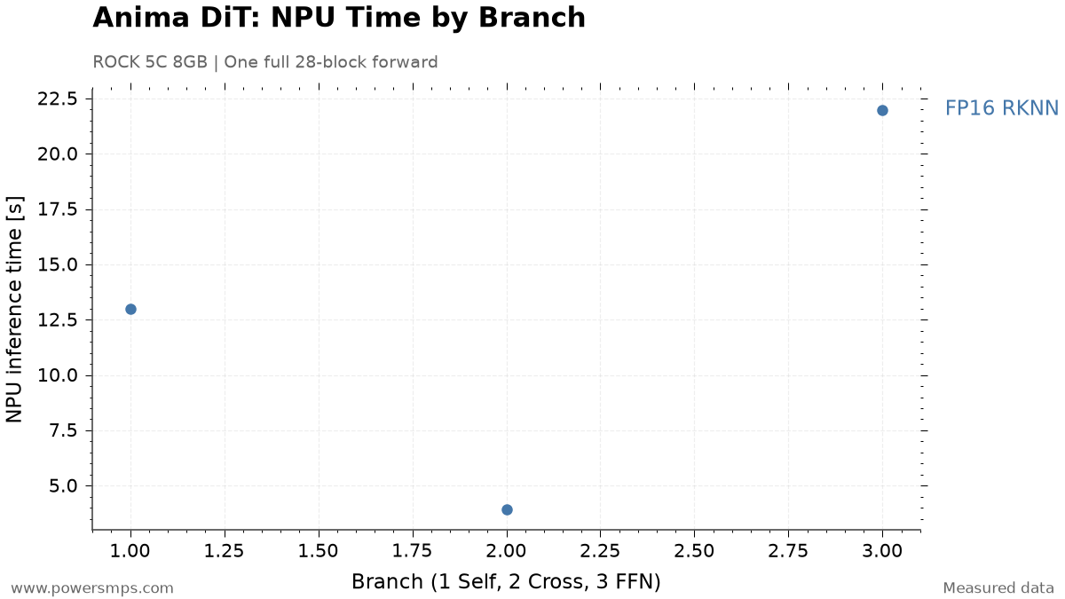
    The average lifecycle latency per model across branches was 0.423 seconds for self-attention, 0.200 seconds for cross-attention, and 0.510 seconds for FFN.

    Under the operating conditions of the 28-step Spectrum sampler, 15 out of the total 28 steps are replaced by extrapolation/prediction, meaning actual NPU operations take place across 13 compute steps. Consequently, when generating 1 image, the total number of lifecycle invocations is 84 models × 13 steps = 1,092 invocations, and cumulative pure lifecycle latency reaches approximately 412.2 seconds.

    If keeping all 84 contexts permanently resident in memory were possible, one could theoretically eliminate the lifecycle overhead for the remaining 12 passes—excluding the initial 1 setup (load/init) and final 1 teardown (release) operations totaling 31.71 seconds.

    \[\Delta T_{\text{theoretical}} = 31.708\,\text{s} \times (13 – 1) = 380.50\,\text{s} \approx 6.34\,\text{분}\]

    According to this calculation, overall generation time could theoretically be reduced from an average of 28.56 minutes (1,713.78 seconds) down to 22.22 minutes (1,333.28 seconds). However, this figure is strictly a theoretical upper bound derived under the premise that keeping 84 contexts resident is physically viable, and does not represent measured or achieved performance in an actual resident denoising pipeline.


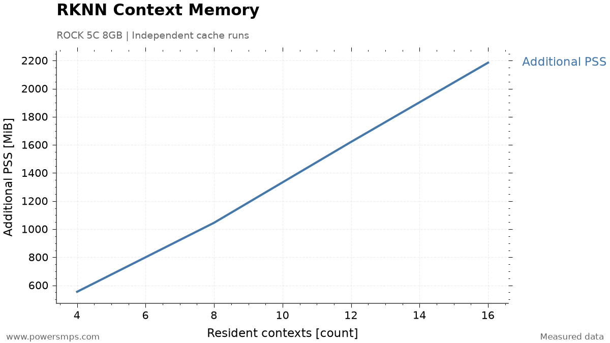
    5. Memory Limits Revealed at 18 Contexts

    We incrementally loaded models into memory one by one, measuring actual memory footprint and swap growth. This experiment was conducted to verify whether an 8GB environment could handle full residency before attempting to execute it.

    Safety abort criteria for the benchmark were defined as available memory (MemAvailable) falling below 1.5 GiB or system swap usage exceeding 16 MiB. Incrementally loading contexts starting from 1 yielded the following results.

    Resident Context Count Process Absolute PSS Additional PSS vs. Baseline MemAvailable Delta System Swap Growth
    1 365.4 MiB 154.9 MiB -151.8 MiB 0 MiB
    4 765.6 MiB 555.1 MiB -558.5 MiB 0 MiB
    8 1,262.6 MiB 1,052.1 MiB -1,000.3 MiB 1.3 MiB
    12 1,823.3 MiB 1,612.8 MiB -1,567.6 MiB 5.0 MiB
    16 2,354.9 MiB 2,144.4 MiB -2,104.2 MiB 9.0 MiB
    18 2,631.4 MiB 2,420.9 MiB -2,372.5 MiB 21.4 MiB (Aborted)

    Upon loading context 18, the absolute process PSS reached approximately 2.57 GiB (2,631.4 MiB), recording an additional PSS over baseline of approximately 2.36 GiB (2,420.9 MiB). System swap increased by 21.4 MiB relative to baseline, triggering early benchmark abortion per safety limits (exceeding 16 MiB). All 18 loaded contexts were immediately and safely released (release wall time: 1.05 seconds), reclaiming device mappings.

    Memory growth occurred not only in host tensors but also in NPU driver device mappings. When sustaining 16 contexts, device mappings accounted for approximately 1.357 GiB, and system swap increased by 19.5 MiB during an 30-second dwell period.

    Linearly extrapolating total resource requirements for all 84 models based on measured memory growth across 16~18 contexts yields the following projections: – Projected device mapping memory: approximately 7.1 GiB – Projected process total additional PSS: approximately 11.3 GiB

    Total physical RAM on the ROCK 5C board is 7.75 GiB. Even before accounting for baseline OS overhead, CPU host-side weights and compute buffers (approx. 0.8~1.0 GiB), and residency space for the prompt encoder and VAE decoder, an additional PSS requirement of 11.3 GiB exceeds hardware limits. Therefore, concurrent residency across all 84 subgraphs fails the memory gate.


    6. Can a Small LRU Cache Solve the Problem?

    If full residency of all 84 models is impossible, one might consider operating a limited context pool of around 4~16 models under an LRU (Least Recently Used) policy, or pinning a select subset of models in memory.

    In fresh standalone processes, allocating pools of 4, 8, 12, and 16 contexts yielded measured additional PSS memory footprints of 554.8 MiB (approx. 0.54 GiB), 1,046.1 MiB (approx. 1.02 GiB), 1,621.5 MiB (approx. 1.58 GiB), and 2,185.4 MiB (approx. 2.13 GiB), respectively.

    Measured additional PSS (MiB) scaling trend according to the number of resident RKNN contexts (4, 8, 12, 16) during standalone process execution on Radxa ROCK 5C 8GB.
    Measured additional PSS (MiB) scaling trend according to the number of resident RKNN contexts (4, 8, 12, 16) during standalone process execution on Radxa ROCK 5C 8GB.

    While additional PSS broadly exhibits an upward trend as contexts increase, the relationship is not strictly linear. Furthermore, this limited caching strategy loses practical utility due to the forward execution structure of the DiT.

    Sequential invocation sequence for step n (total 84 models)
    [Model 00 (self) → Model 01 (cross) → Model 02 (FFN) → ... → Model 83 (FFN)]
      ↓ Residual connection accumulation and scheduler latent update
    Sequential invocation sequence for step n+1 (identical pass across all 84 models)
    [Model 00 (self) → Model 01 (cross) → Model 02 (FFN) → ... → Model 83 (FFN)]
    

    Each branch output in a DiT block is immediately summed into the host’s FP32 residual stream and fed as input to subsequent branches and blocks. Furthermore, only after all 84 branch operations complete can the sampler update the denoising latent representation and advance to the next diffusion step. That is, loop interchange to reorder invocations is impossible due to sequential dependencies between models.

    Structurally, all 84 models are cyclically referenced in fixed order 1 times per 1 step. Before the same model can be re-invoked, 83 other models must be evaluated. Therefore, under any standard LRU cache with capacity strictly below 84 (e.g., capacity 4, 8, 16, 28, 56, etc.), every loaded model is inevitably evicted just before it could ever be reused: – LRU simulation result: across a total of 1,092 invocations, 0 hits / 1,092 misses (0% cache hit rate)

    Even if static pinning were applied to keep select models (e.g., model 0~15) in memory without eviction, the maximum time savable across 16 models amounts to only 16 model’s lifecycle per compute step. For 1 image, this reaches an absolute theoretical maximum savings of only approximately 72.4 seconds—which is not an empirically verified measurement. In return, the price paid is an additional PSS overhead of 2.13 GiB (2,185.4 MiB) and swap churn during sustained retention. Sacrificing system stability and inducing swap jitter for a modest theoretical saving of 72.4 seconds represents an unsound engineering trade-off.


    7. Configuration Maintained on 8GB

    The core bottlenecks and empirical findings derived from the W8A8 FFN integer quantization and resident context cache experiments are summarized below:

    • FFN W8A8 quantization: Computation accelerated, but fell short of visual quality standards.
    • Full model residency: Swap activity increased at 18 contexts, and additional PSS for 84 resident models extrapolated to approximately 11.3 GiB.
    • Limited caching: Under cyclic invocations, models were evicted before reuse, yielding zero LRU cache hits.

    On the ROCK 5C 8GB, we retained the FP16 models and chose an on-demand strategy: staging and executing each required model sequentially, followed immediately by release. In this comparison, the memory penalty far outweighed the latency benefits of keeping models resident.

    This decision applies specifically to this 8GB board and partitioned configuration. If memory capacity or model partitioning strategies change, the trade-offs of residency must be re-evaluated.

    Instead of stacking models in memory, can the graph partitioned into 84 subgraphs be consolidated into fewer models? In Part 4, we upgrade the compiler version to attempt graph operator fusion and compare latency and memory trade-offs.

  • RKNN Toolkit 2.3.2 vs 2.3.0: AdaLN Compiler Crash and Operator Fusion Benchmark

    RKNN Toolkit 2.3.2 vs 2.3.0: AdaLN Compiler Crash and Operator Fusion Benchmark

    Affiliate Disclosure: This post contains AliExpress affiliate links. If you make a purchase through these links, the author may receive a commission.


    1. Can Partitioned DiT Blocks Be Recombined?

    When deploying generative Diffusion Transformers (DiT) in embedded NPU environments, runtime memory limits and operator support constraints are critical factors directly dictating architectural design. This in-depth experiment was conducted on 2026-8-20 on a Radxa ROCK 5C 8GB single-board computer.

    The experiment used a directly purchased ROCK 5C 8GB board.

    The test board is a RK3588S2-based ROCK 5C, and the RKNN target is rk3588. It should be distinguished from the ROCK 5C Lite listed on the same product page.

    In Part 1, the Anima configuration partitioned the 28 DiT blocks into attention, cross-attention, and FFN components, yielding 84 FP16 RKNN models, with AdaLN and residual additions handled on the CPU. Here, we examined whether the 3 models per block could be fused into a single model.

    The baseline pipeline processed AdaLN (Adaptive LayerNorm) operations and residual additions in the host CPU Python runtime. However, repeatedly loading, executing, and releasing 3 subgraphs per step within a single DiT block—round-tripping intermediate tensors to the CPU host—incurs substantial driver overhead. If self-attention, cross-attention, FFN, and AdaLN within a block could be fused into a single RKNN graph (a fused 1-model), we expected to reduce the lifecycle invocations per block from 3 to 1 while eliminating host tensor transfer overhead.

    However, compiling a graph containing AdaLN operators under RKNN Toolkit 2.3.2—the default compiler at the time—triggered a fatal compiler segmentation fault (SIGSEGV, exit code 139). We first had to determine whether this crash stemmed from fundamental hardware non-support for the Anima DiT architecture or a compiler bug.


    2. Building the Same AdaLN Graph with Different Toolkits

    To isolate the compiler crash, we extracted a minimal ONNX reproducer containing only the crashing AdaLN operator instead of the full DiT block and ran compilation experiments.

    We compiled the identical AdaLN reproducer graph using RKNN Toolkit 2.3.2 and 2.3.0. All other build conditions were kept constant to compare results across compiler versions.

    Using the identical reproducer ONNX model, target (rk3588), and single-core optimization settings, the build results were as follows:

    Toolkit VersionAdaLN Graph BuildExit Code
    2.3.2Failed: SIGSEGV139
    2.3.0Success0

    In 2.3.2, the build aborted with a SIGSEGV immediately following LayerNorm graph optimization. In 2.3.0, the identical graph built without errors.

    Because the outcome differed solely by version on identical input graphs and targets, we determined this failure to be a compiler regression. The older 2.3.0 release provided a functional workaround for this graph, rather than resolving the issue by upgrading to a newer release.


    3. Verifying Fused Model Execution at 64px and 512px

    Using Toolkit 2.3.0, we compiled a fused model for the first DiT block and verified both a 64px test configuration and a 512px production inference configuration.

    Fused Block ResolutionRKNN ConversionOn-Board Execution
    64pxSuccessInit and inference verified
    512pxSuccessInit, inference, and release verified

    The 512px model build completed without triggering system swap. However, because certain Transpose and Erf operations were offloaded to the CPU, fusing into a single RKNN file does not mean every operator executes entirely on the NPU.

    A more critical validation checkpoint was binary compatibility with the target board’s local runtime. Even if compiled with 2.3.0, deployment complexity escalates sharply if the board OS’s RKNPU kernel driver or runtime libraries must be forcibly replaced.

    The compiled model was executed under runtime API 2.3.0 and driver 0.9.8. Without modifying the kernel or driver, we verified loading, initialization, inference, and context release across 3 repeated rounds of conditional and unconditional inference.

    In this single-block validation, switching only the compiler environment was sufficient to execute on the existing board runtime.


    4. Numerical Differences in Single-Block Output

    Once hardware execution of the fused model was verified, we performed a single-block correctness gate to confirm whether the NPU fused operation numerically matched the original floating-point reference tensors. The references used were the original PyTorch FP16 block outputs and ONNX Runtime (ORT) outputs.

    Target Architecture Reference Tensor Cosine Similarity Max Absolute Error (Max Abs) Mean Absolute Error (Mean Abs) Mean Squared Error (MSE) NaN/Inf Detection
    64px Fused PyTorch 0.99998315 0.28125 0.0018879 4.2748e-05 0 / 0
    64px Fused ONNX Runtime 0.99998608 0.28125 0.0018948 3.5387e-05 0 / 0
    512px Split (Baseline) PyTorch 0.99999881 0.14937 0.0002283 1.0841e-06 0 / 0
    512px Fused (Candidate) PyTorch 0.99997673 0.25000 0.0011279 2.1100e-05 0 / 0
    512px Fused (Candidate) ONNX Runtime 0.99997590 0.28906 0.0011662 2.1854e-05 0 / 0

    The 512px fused model recorded a cosine similarity of 0.99997673 and a maximum absolute error of 0.25000 against the PyTorch reference output, with no NaNs or Infs detected.

    However, the fused model’s MSE was 2.1100e-05, roughly 19.5 times higher than the 1.0841e-06 of the baseline split architecture. High cosine similarity on a single block alone cannot guarantee the image quality of the final output after traversing all 28 blocks over multiple steps.


    5. Fewer Context Invocations, but Only a 0.47% Speedup

    The primary motivation for pursuing subgraph fusion was latency reduction. We anticipated measurable speedups by migrating AdaLN and residual operations from host Python into the compiled graph, thereby reducing driver context invocations.

    On the ROCK 5C board, we executed 3 rounds of a 2-pass Classifier-Free Guidance (CFG) computation stream for a 512px single block and precisely measured the average execution time of each stage.

    512px DiT single-block measured component breakdown. 1=load, 2=init, 3=inference×2, 4=release, 5=host AdaLN/residual. Component total is Split 4.3856 s, Fused 4.3650 s.
    Comparison of component latency breakdown between Split 3-Model baseline and Fused 1-Model candidate for 512px single block on Radxa ROCK 5C.

    The table below compares measured latency stage-by-stage between the baseline 3-model split configuration and the candidate Fused 1-model configuration.

    Execution Stage & Component Baseline 3-Model Split Candidate Fused 1-Model Fused Delta Cause of Change & Analysis
    Model Load 0.4863 s 0.4814 s -0.0049 s Weight file loading time (marginal reduction for a single block)
    Runtime Init 0.4464 s 0.4240 s -0.0224 s Slight reduction in NPU runtime context initialization time
    NPU Inference (×2) 3.1177 s 3.2972 s +0.1795 s (+5.76%) NPU execution slowdown due to operator fusion
    Context Release 0.1694 s 0.1623 s -0.0071 s Context memory release time
    Host AdaLN & Residual 0.1658 s 0.0000 s -0.1658 s (-100%) Elimination of separate Python host AdaLN path
    Net Component Sum 4.3856 s 4.3650 s -0.0206 s (-0.47%) Actual net time saved was merely 0.0206 s
    Measured Wall Time 4.7379 s 4.4981 s -0.2398 s (-5.06%) Includes instrumentation distortion from multiple memory snapshots in split mode

    The benchmark data revealed bottlenecks that ran counter to intuitive expectations. First, host compute time of 0.1658 s was completely eliminated to 0 s in the Fused model. However, pure NPU forward inference time (Inference ×2) increased by +0.1795 s (+5.76%) from 3.1177 s to 3.2972 s. The increased inference latency in the fused configuration completely offset the savings gained by removing host compute (0.1658 s).

    Second, while context invocations dropped by 66.7% from 3 to 1, lifecycle overhead (Load, Init, Release) did not decrease as expected. Total single-block lifecycle time fell only by 3.1% from 1.1021 s to 1.0678 s. This revealed that practical RKNPU driver initialization and loading overhead is governed by total model file weight footprint (approximately 140~155 MB) and graph complexity rather than raw C API call counts.

    Third, while measured wall time appeared to decrease by 0.2398 s (5.06%), this figure included profiling overhead from collecting memory snapshots 6 times across 3 sub-contexts in split mode. Excluding snapshot measurement distortion, the actual net speedup based on pure component totals was merely 0.0206 s (-0.47%) per block.


    6. NPU Device Mapping Memory Increased by 94.30 MiB

    While the latency reduction was negligible, runtime memory suffered significant penalties. The memory metrics measured at the board level were as follows:

    Memory Metric Baseline 3-Model Split Candidate Fused 1-Model Difference & Rate of Change
    NPU Device-Mapped Device PSS 127,144 KiB 223,704 KiB +96,560 KiB (+94.30 MiB, +75.9%)
    Peak Process PSS During Execution 648,282 KiB 694,882 KiB +46,600 KiB (+45.51 MiB, +7.2%)
    New System Swap Generated 0 0 0 (Safe for single block)

    The split architecture executes each branch sequentially before releasing it. The peak NPU device mapping maintained at any one time was 127,144 KiB, or approximately 124.16 MiB.

    The fused architecture retains the entire block within a single runtime context. Device mapping increased to 223,704 KiB—approximately 218.46 MiB—consuming an additional 94.30 MiB.

    On the ROCK 5C sharing 8GB of total LPDDR4X memory—where the background OS, text encoder, and VAE must coexist—a 75.9% surge in device-mapped memory introduces severe system pressure.


    7. Why Operator Fusion Was Not Adopted

    Extrapolating single-block differences across the complete pipeline suggested an estimated reduction of approximately 7.51 s. This estimate was not measured by running full image generation.

    • Speed: Reductions in host compute were largely cancelled out by increased NPU inference latency.
    • Memory: Executing the same block required higher device-mapped memory.
    • Precision: Although single-block cosine similarity was high, MSE was larger than in the baseline split configuration.

    Because speedup was capped at 0.47% while memory consumption expanded, we retained the baseline split architecture for this board.

    The verification scope was limited to a single block. These findings do not reflect experiments fusing all 28 blocks to generate complete images or prolonged operational testing.

    Both the residency experiment in Part 3 and this fusion experiment demonstrated that reducing call counts alone cannot account for overall performance. NPU compute time and memory overhead must be evaluated together to choose optimizations viable on a 8GB board.

  • Generating Anima Images on RK3588: RKNN Conversion and Execution on ROCK 5C 8GB

    Generating Anima Images on RK3588: RKNN Conversion and Execution on ROCK 5C 8GB

    Affiliate Disclosure: This post contains AliExpress affiliate links. If you make a purchase through these links, the author may receive a commission.

    1. Running Anima on ROCK 5C 8GB

    With 8GB of memory, the Radxa ROCK 5C 8GB single-board computer (SBC) was used to verify on-device execution of a multi-billion-parameter Diffusion Transformer (DiT) model.

    The main processor of the board is a Rockchip RK3588S2 SoC, and its dedicated Rockchip NPU runtime target is rk3588. In the same manufacturer’s Radxa ROCK 5C product line, the Lite model with the RK3582 option uses a different chipset with scaled-down NPU units and CPU core configurations. Therefore, to reproduce this 8GB DiT compute pipeline, one must verify the RK3588S2-based ROCK 5C 8GB model.

    The DiT responsible for Anima’s image generation consists of 28 blocks. In this experiment, we partitioned and converted it into a format executable on the NPU of the ROCK 5C.

    The fixed I/O specifications for the on-device conversion are as follows: – Batch size: 1 – Generation resolution: 512×512 pixels – Input token specification: 1024 image tokens, 512 text conditioning tokens – Target ONNX version: Opset 19

    Qwen3 was used for text encoding, and Qwen-Image VAE was used for image reconstruction. In this configuration, the primary DiT compute is handled by the NPU, while text encoding and VAE decoding are handled by the CPU.


    2. Why the DiT Was Partitioned into 84 RKNN Models

    Packaging all 28 blocks of the DiT architecture into a single monolithic RKNN model ran into structural limitations of the RKNN compiler. In our 2026-8 experiments using the RKNN-Toolkit2 2.3.2 environment, compiling the entire DiT block or building branches combined with AdaLN (Adaptive Layer Normalization) operations caused a native segfault (exit 139).

    Decomposing the graph down to minimal units for debugging revealed that while large Linear layers or standard GELU FFN graphs compiled properly for the NPU target, subgraphs containing the AdaLN LayerNorm + broadcast shift/scale/gate pattern consistently triggered the same segfault regardless of weight size. This confirmed that the issue was not out-of-memory, but a compiler error in parsing specific graph operator patterns.

    We separated the 3 compute branches that can execute on the NPU in each DiT block, handling normalization, gating, and residual summation on the CPU.

    Each of the 28 DiT blocks was divided into 3 subgraphs: self-attention, cross-attention, and FFN. Self-attention computes relationships between image tokens, cross-attention computes relationships between text conditioning and image tokens, and FFN transforms the features of each token.

    DiT block architecture alternating between blue CPU stages and orange NPU stages. The CPU handles AdaLN, gate multiplications, and FP32 residual accumulation for each branch, while the NPU processes FP16 self-attention, cross-attention, and FFN.
    CPU/NPU execution sequence for a single DiT block. The NPU processes FP16 attention and FFN, while the CPU handles AdaLN before each branch, gate multiplications after each branch, and FP32 residual accumulation. This structure repeats across 28 blocks.

    A total of 84 (28 × 3) FP16 RKNN models were generated, totaling approximately 3.99GB in size. AdaLN, gate multiplication, RoPE, input/timestep embeddings, and final projection were executed on the CPU. Residual accumulation was maintained in FP32.

    • Separate operations to be handled by the CPU from operations to be handled by the NPU in the original model.
    • Convert NPU operations into fixed-I/O-shape ONNX graphs and then compile them to RKNN.
    • Compare single-block and full-block outputs against the original model before running image generation.

    3. How Close Are the Outputs Before and After Conversion

    The most critical step in hybrid partitioned conversion is preventing numerical error accumulation across frameworks. We separated verification into single-block validation and sequential cumulative validation across all 28 blocks.

    Single-Block Comparison

    We compared ONNX and RKNN outputs against the original PyTorch block’s FP16 branch operations and FP32 residual accumulation. This step verifies whether the converted operations produce outputs pointing in the same direction as the original model.

    Comparison Target Cosine Similarity (Cosine) Mean Absolute Error (MAE) Maximum Absolute Error (Max AE) NaN / Inf Occurrences
    PyTorch → ONNX 0.9999994183 0.00012350 0.09396 0 / 0
    PyTorch → RKNN 0.9999990896 0.00019535 0.11446 0 / 0
    ONNX → RKNN 0.9999995474 0.00014175 0.06969 0 / 0

    The cosine similarity between the baseline PyTorch output and the RKNN output was 0.9999990896. For a single block, the outputs before and after conversion maintained highly aligned trajectories.

    Output Comparison Across 28 Blocks

    To confirm that numerical errors do not amplify while passing from Block 0 through Block 27 across all 28 blocks, we compared the pure ONNX accumulated tensor against the RKNN 84-core accumulated tensor.

    • Lowest single-block cosine similarity: 0.999993668 (lowest among all 28 blocks)
    • Final hidden layer similarity (Hidden Cosine): 0.9999989412
    • Final 16-channel prediction tensor similarity (Final Prediction Cosine): 0.9999989072
    • Final prediction tensor MAE: 0.00129712
    • Final prediction tensor Max AE: 0.00830078
    • Boundary NaN / Inf occurrences: 0

    Even after passing through 28 blocks, no NaNs or Infs occurred, and high similarity to the reference output was preserved. However, this numerical comparison must be distinguished from the perceptual quality evaluation of the final generated image.


    4. How Long Did Denoising Take?

    Pure NPU Latency by Branch Across Full 28-Block Forward Pass

    On the RK3588 NPU, the total pure inference time for a single forward pass through all 28 DiT blocks is approximately 38.90 seconds. The branch-by-branch values below represent the summed execution times across all 28 blocks.

    The detailed latency breakdown by core is as follows: – Self-Attention Core: 12.99 seconds – Cross-Attention Core: 3.92 seconds – FFN Core: 21.99 seconds

    NPU inference time sum by branch in a single full DiT forward pass on the ROCK 5C across all 28 blocks. 1: self-attention, 2: cross-attention, 3: FFN. Not single-block latency.
    NPU inference time sum by branch in a single full DiT forward pass on the ROCK 5C across all 28 blocks. 1: self-attention, 2: cross-attention, 3: FFN. Not single-block latency.

    The parameter-heavy FFN core accounts for approximately 56.5% of total pure NPU inference time. Note that the total wall-clock time for the full 28-block test accompanied by ONNX numerical validation logic was 162.8 seconds, which is distinct from the pure NPU compute time (38.90 seconds).

    20-Step Sequential CFG Denoising Results

    We executed the actual image generation workflow—a 20-step sequential Classifier-Free Guidance (CFG, guidance scale 4.0) denoising process—directly on the board. Due to memory constraints, conditional (positive) and unconditional (negative) predictions were not batched together, but processed via sequential invocations.

    • 20-step denoising: 2,408.54 seconds
    • Per-step average: 120.40 seconds
    • Pure NPU compute per step: 76.21 seconds
    • Model staging, host processing, etc. per step: approx. 44.19 seconds
    • NaN/Inf occurrences across all 20 steps: 0

    The approximately 44.19 seconds of non-NPU overhead per step includes loading, initialization, and releasing (load/init/release) across the 84 RKNN models, as well as host computation and boundary marshalling costs. Subsequent optimizations will isolate and profile these components individually.


    5. Reducing Image Reconstruction Time by Replacing the VAE

    The VAE decoding process, which reconstructs the denoised latent representation into a 512×512 pixel RGB image, poses a heavy CPU compute burden. Using the official Diffusers Qwen-Image VAE FP32 CPU implementation as-is resulted in a decoding latency of 2,154.51 seconds (approx. 35 minutes 54 seconds), introducing a severe bottleneck on par with the total 20-step DiT denoising time.

    For VAE decoding, we applied an ARM NEON- and OpenMP-optimized CPU implementation from stable-diffusion.cpp. Rather than re-initializing the text encoder and transformer, the pipeline was linked to receive only the post-denoised latent tensor and reconstruct the image.

    Configured with 4 CPU threads, a tile size of 32×32, and an overlap of 0.5, the comparison results between VAE backends are as follows:

    Metric Official Diffusers FP32 VAE sd-cpp Tiled CPU VAE Improvement
    Decoding Latency 2,154.51 seconds 155.04 seconds 13.90× faster (1,999.47 seconds saved)
    PSNR (vs. Diffusers Output) Baseline 31.444 dB Compared to reference
    11×11 Gaussian SSIM 1.00000 0.96109 Compared to reference
    Output Resolution & Format 512×512 RGB 512×512 RGB NaN / Inf: 0

    Visual inspection confirmed that composition, color, and fine details were well preserved. While PSNR and SSIM do not imply identical outputs, decoding time was reduced to the 2 minutes 35 seconds range.

    Total Latency: Denoising Plus Image Reconstruction

    Integrating VAE acceleration yields the following overall image generation latency: – DiT 20-step sequential CFG denoising: 2,408.54 seconds – sd-cpp tiled VAE decoding: 155.04 seconds – Total generation time (excluding 1-time prompt encoding): 2,563.58 seconds (approx. 42 minutes 44 seconds)


    6. The Next Bottleneck: Denoising

    By reducing VAE decoding latency from 2,154.51 seconds to 155.04 seconds, the VAE’s share of overall pipeline latency dropped dramatically from 47.2% to 6.0%. Consequently, the dominant system bottleneck shifted to DiT 20-step denoising (2,408.54 seconds, 94.0% of the total).

    Deconstructing DiT denoising internally shows that pure NPU compute takes 76.21 seconds per step (across 20 steps, totaling 1,524.20 seconds), while the remaining approximately 884.34 seconds consists of non-NPU overhead including model lifecycle and host processing. Context residency was considered as a candidate to eliminate repetitive initialization costs, but memory headroom and actual savings required independent verification under an 8GB environment. Those experimental results are covered in Part 3.

    Subsequent optimizations examined compute iteration count alongside memory usage. Part 2 covers reducing compute steps with Spectrum, while Part 3 explores the limits of quantization and model residency against image quality and memory constraints. In Part 4, we evaluate compiler version differences and the trade-offs of graph operator fusion.

  • 3.3V MCU Relay Driver MOSFET Selection: On-Resistance, Gate Resistor, and Voltage Rating Calculations

    3.3V MCU Relay Driver MOSFET Selection: On-Resistance, Gate Resistor, and Voltage Rating Calculations

    When using a 3.3V GPIO to control a 12V relay, you must first check the guaranteed on-resistance at the actual gate voltage rather than the MOSFET threshold voltage. Calculating the load current determined by power supply and coil tolerances, the drain peak voltage during coil turn-off, and the GPIO charge and discharge currents provides a clear rationale for component selection.

    The following is a low-speed DC relay ON/OFF design example based on assumed operating conditions, not empirical measurements from a specific product.

    1. Check Guaranteed On-Resistance Instead of VGS(th)

    In the AO3400A datasheet Rev 3.1, the threshold voltage VGS(th) is defined under the conditions of drain current 250µA and VDS=VGS. The minimum, typical, and maximum values are 0.65V, 1.05V, and 1.45V, respectively. This test current is a conduction current used to define the threshold, not a condition that guarantees low on-resistance at relay load currents.

    The manufacturer’s maximum on-resistance specifications are as follows. The junction temperature condition for the table is TJ=25°C.

    Gate Voltage VGS Test Drain Current Maximum RDS(on)
    2.5V 3A 48mΩ
    4.5V 5A 32mΩ
    10V 5.7A 26.5mΩ

    Even when using a 3.3V MCU, the GPIO High output is not always 3.3V. You must check the minimum VOH and load conditions in the MCU datasheet, and verify that VGS—accounting for voltage drops across the gate resistor network and source voltage fluctuations—is sufficiently higher than the test voltage specified in the on-resistance rating. Furthermore, the test currents in the on-resistance table must not be interpreted as allowable continuous currents on an actual PCB.

    Source: AO3400A Official Datasheet, electrical characteristics and thermal characteristics tables.

    2. Coil Current and Conduction Loss Calculations

    The example conditions are assumed as follows. The GPIO values are not guaranteed specifications of any specific MCU.

    Item Example Assumption
    Nominal coil voltage and resistance 12V·120Ω
    Maximum supply voltage 13.2V
    Minimum coil resistance considering low temperature and tolerance 108Ω
    Minimum GPIO VOH 2.9V
    Gate charging current budget 4mA
    On-resistance used for calculation 48mΩ, VGS=2.5V·TJ=25°C specification

    The nominal current is 12V/120Ω=100mA, and the assumed maximum current is as follows:

    \[I_{coil,max}=\frac{13.2}{108}\approx0.12222\ \mathrm{A}\]

    Conduction loss is proportional to the square of current:

    \[P_{cond}=I_{coil}^{2}R_{DS(on)}\]

    The calculated value at nominal current is 0.100²×0.048=0.00048W, or 0.48mW. Under the assumed maximum current condition, it is approximately 0.12222²×0.048=0.000717W, or 0.717mW.

    This value is a conduction loss calculation applying the 25°C on-resistance. It is not a final guaranteed temperature value that includes on-resistance increases at high temperatures, switching losses, and actual PCB heat dissipation conditions. Because datasheet thermal characteristics are based on a 2oz copper, 1in² FR4 board in still air, actual board conditions must be verified separately.

    Normalized conduction loss according to current ratio and on-resistance ratio. Resistance multipliers 1.0, 1.3, and 1.5 are assumptions for comparison and not guaranteed values at specific temperatures.
    Normalized conduction loss according to current ratio and on-resistance ratio. Resistance multipliers 1.0, 1.3, and 1.5 are assumptions for comparison and not guaranteed values at specific temperatures.

    The resistance multipliers 1.0, 1.3, and 1.5 in the graph are model values chosen for comparison. They are not manufacturer-guaranteed values or measured data corresponding to specific temperatures. Under the same on-resistance, the graph shows the relationship where conduction loss increases by a factor of 1.44 when the current increases by a factor of 1.2.

    3. GPIO, Gate, and Relay Interconnection Conditions

    3.3V GPIO, 1kΩ gate resistor, 47kΩ pull-down, and AO3400A MOSFET circuit driving a 12V relay. A flyback diode is connected across the coil, and ground is shared.
    Low-side drive example for a 12V·120Ω relay coil. The cathode of the flyback diode is connected to +12V. Review component values together with the selection criteria in the main text.

    The example is a low-side N-MOSFET circuit where the MCU and load supply share a common ground. Connections are listed in the following table:

    Device / Node Connection
    Relay coil Between +12V and Q1 drain
    Q1 source Common GND shared with MCU
    Series gate resistor Rg Between GPIO and Q1 gate, example value 1kΩ
    Pull-down resistor Rpd Between Q1 gate (downstream of Rg) and source, example value 47kΩ
    Flyback diode D1 Cathode to +12V, anode to Q1 drain

    The body diode of a low-side N-MOSFET conducts from source to drain. When the coil is turned off and the drain flies up to a positive voltage higher than the supply, the body diode is reverse-biased and cannot substitute for the coil flyback freewheeling path.

    The relationship between diode ratings and relay release time can be further referenced in the previous article, Relay Flyback Diode Selection and Turn-Off Time Calculations.

    4. Series Gate Resistor and Pull-Down Calculations

    Modeling the GPIO as an ideal 3.3V voltage source and budgeting an initial gate charging current of 4mA, the lower limit calculation for the external series resistance is 3.3V/4mA=825Ω. In the example, 1kΩ is selected. Neglecting the GPIO internal output resistance, the calculated initial current upper limit is 3.3V/1kΩ=3.3mA. For actual component selection, verify both recommended source/sink currents and VOH/VOL conditions in the MCU datasheet. Never use the absolute maximum rated current as a continuous driving target.

    Connecting a 47kΩ pull-down behind the gate creates voltage division in steady state. Under the conditions of minimum VOH 2.9V, negligible gate leakage, and a common ground without source voltage bounce, the calculation is as follows:

    \[V_{GS}=2.9\times\frac{47}{1+47}\approx2.8396\ \mathrm{V}\]

    Under this DC assumption, the voltage is higher than the test voltage for the 2.5V on-resistance specification. In practical circuits, verify margin across temperature, supply tolerances, and source voltage variations. When the GPIO outputs 3.3V, the DC current flowing through the resistor network is 3.3V/48kΩ=68.75µA.

    A static calculation is also possible for when the GPIO is High-Z during reset. Assuming a total leakage current of 1µA and an allowable gate voltage of 0.3V, Rpd≤0.3V/1µA=300kΩ. With 47kΩ, the static leakage voltage is approximately 47mV. While the pull-down should be placed close to the gate, this calculation does not guarantee prevention of false turn-on caused by Miller current injection during rapid drain voltage changes or across all power sequencing conditions.

    5. MOSFET Voltage Rating Calculations with Coil Clamping

    The absolute maximum VDS rating of the AO3400A is 30V. When selecting a device, adequate design margin must exist for the following voltage sum:

    \[V_{sup,max}+V_{clamp,max}+V_{overshoot} < V_{DS,rating}\]

    Assuming a clamp voltage of 1V for a standard diode and a wiring overshoot of 3V, the peak is 13.2+1+3=17.2V. Although this is lower than 30V, this confirms only the assumed voltage sum, so actual drain waveforms and component tolerances must be verified.

    Conversely, in an assumption combining a 24V Zener and a 0.8V forward-voltage diode, even without overshoot the sum is 13.2+24+0.8=38V. Therefore, the 30V AO3400A cannot be used under these conditions. When selecting higher voltage-rated devices, evaluate based on the Zener’s actual clamp current, temperature, tolerance, and wiring surges. Sizing MOSFET voltage rating based solely on supply voltage makes it easy to overlook this difference.

    6. Distinguishing and Validating Low-Speed ON/OFF vs. PWM

    The total gate charge Qg of the AO3400A is typical 6nC and maximum 7nC, but the test conditions are VGS=4.5V, VDS=15V, and ID=5.7A. This must not be used as a guaranteed charge value under 3.3V drive. Furthermore, Qg/Ig is a coarse charging time estimate and does not equal the actual drain transition time including the Miller plateau. For relevant principles, refer to the TI SLUA618A Gate Driver Design Document.

    Do not apply resistor values for low-speed relay ON/OFF directly to high-speed PWM solenoid circuits. Whether a dedicated driver is required should be determined by examining gate charge, GPIO source/sink capability, switching losses, temperature, and the EMI budget together.

    The final verification sequence is as follows:

    1. Recalculate maximum current using actual component coil tolerances and supply voltage ranges.
    2. Measure gate-to-source voltage during normal operation to verify it meets the on-resistance guarantee condition.
    3. Check for spurious gate turn-on and source voltage bounce during boot, reset, and power-up sequencing.
    4. Verify that the drain peak and ringing during coil turn-off remain within the selected breakdown voltage margin.
    5. Check heat dissipation on the actual PCB and at operating temperatures.

    The core sequence is Verify guaranteed on-resistance at actual VGS → Calculate maximum coil current and losses → Validate gate resistor network → Verify VDS including clamp. The 1kΩ and 47kΩ in this example are a starting point calculated under these conditions, and must be reconfirmed against the datasheets of the MCU and relay to be used.